Clustering is an unsupervised learning technique that can help you uncover hidden patterns in your time series data.
Scikit-learn has a wide range of clustering algorithms, including K-means, DBSCAN, and Agglomerative Clustering.
In this tutorial, we’ll explore how to use K-means with different transformations to cluster time series data.
Using the right data transformations can help you get your desired results faster than just trying different clustering algorithms over the same data.
To use other clustering algorithms, you can follow the same steps, just change the algorithm object.
Let’s get started!
Loading The Data With Pandas
First things first, we need to load our data.
In this tutorial, we’ll be using a dataset containing website traffic data from lacity.org.
The dataset contains information like date, device category, browser, and the number of sessions.
Sessions are periods of time when a user is actively using the website.
Usually they are measured by looking at user activity and have a timeout after 30 minutes since the last user action.
For example, right now you are in a session on my website. If you leave the page and come back after 2 hours, you will be in a new session.
Let’s start by loading the data using pandas:
import pandas as pd
import os

path = 'path/to/your/dataset'
data = pd.read_csv(os.path.join(path, 'lacity.org-website-traffic.csv'),
                   parse_dates=['Date']).loc[:, ['Date', 'Device Category', 'Browser', 'Sessions']]
| Date | Device Category | Browser | Sessions | unique_id | |
|---|---|---|---|---|---|
| 0 | 2014-01-01 00:00:00 | desktop | Chrome | 934 | desktop_Chrome |
| 1 | 2014-01-01 00:00:00 | desktop | Firefox | 761 | desktop_Firefox |
| 2 | 2014-01-01 00:00:00 | desktop | Internet Explorer | 1107 | desktop_Internet Explorer |
| 3 | 2014-01-01 00:00:00 | desktop | Opera | 35 | desktop_Opera |
| 4 | 2014-01-01 00:00:00 | desktop | Safari | 554 | desktop_Safari |
Now, we need to reshape the data into a wide format, where each row represents a unique combination of device category and browser.
In other words, each of our rows needs to represent a single time series.
We want to cluster time series, so each of them becomes a data point.
We’ll create a new column unique_id for this purpose:
data['unique_id'] = data['Device Category'] + "_" + data['Browser']
wide_df = data.groupby(['Date', 'unique_id']).sum().unstack().T.fillna(0).reset_index(level=0, drop=True)
wide_df.head()
| unique_id | 2014-01-01 00:00:00 | 2014-01-02 00:00:00 | 2014-01-03 00:00:00 | 2014-01-04 00:00:00 | 2014-01-05 00:00:00 |
|---|---|---|---|---|---|
| desktop_“mozilla | 0 | 0 | 0 | 0 | 0 |
| desktop_‘Mozilla | 0 | 0 | 0 | 0 | 0 |
| desktop_(not set) | 0 | 0 | 0 | 0 | 0 |
| desktop_AdobeAIR | 0 | 0 | 0 | 0 | 0 |
| desktop_Bluebeam Revu Browser - cef version: 57.0.0.0 | 0 | 0 | 0 | 0 | 0 |
Great! Now that we’ve got our data in the desired format, let’s move on to the clustering part.
Raw Time Series Clustering
We’ll use scikit-learn’s K-means clustering algorithm to group our time series data.
K-means clustering is a distance-based algorithm, which means it calculates the distance between data points to group them into clusters.
When working with time series data containing different scales or units, it’s important to preprocess the data to ensure that the algorithm captures patterns that are independent of the scale.
For example, consider data for people using Chrome on a desktop and people using Opera on a mobile device.
The number of sessions for the former will be much higher than the latter, but our objective is to cluster the patterns together independent of the scale.
To achieve this, we’ll preprocess the data using MaxAbsScaler, which scales the data by its maximum absolute value.
The reason for choosing MaxAbsScaler over StandardScaler is that some series in our dataset have a lot of zeros, making the data sparse.
Using StandardScaler would break the sparse structure of the data, which is usually not desirable.
However, you can use whichever scaler you prefer or the one that works best for your data.
from sklearn.cluster import KMeans
from sklearn.preprocessing import MaxAbsScaler

prep = MaxAbsScaler()
kmeans = KMeans(n_clusters=4, random_state=0)

scaled_data = prep.fit_transform(wide_df)
kmeans.fit(scaled_data)
We import the objects we need to scale and cluster the data from sklearn.
Then we create an instance of the MaxAbsScaler class, which will be used to preprocess our data before fitting the clustering model.
Next, we create an instance of the KMeans class with n_clusters=4, specifying that we want to group the data into four clusters.
We also set the random_state parameter to 0, which ensures that the algorithm’s random initialization is consistent every time the code is run.
This helps in obtaining reproducible results.
I set the n_clusters parameter to 4, but you can choose any number of clusters you want.
I will talk more about choosing the right number of clusters in the next section.
The fit_transform method of the MaxAbsScaler first fits the scaler to the data (i.e., learns the maximum absolute values of each feature) and then transforms the data by scaling it according to the learned values.
The transformed data is returned as a new Numpy array.
The fit method of the KMeans class fits the K-means clustering model to the data, learning the optimal cluster centroids.
Selecting The Best Number Of Clusters
We can see which time series belong to which cluster by using the labels_ attribute of the kmeans object:
This attribute contains the cluster to which each time series (row) belongs.
for cluster in range(kmeans.n_clusters):
    print(f"Cluster {cluster}")
    cluster_data = wide_df[kmeans.labels_ == cluster]
    for i in range(min(5, cluster_data.shape[0])):
        print(cluster_data.index[i])
    print()

Cluster 0
desktop_"mozilla
desktop_'Mozilla
desktop_(not set)
desktop_AdobeAIR
desktop_Bluebeam Revu Browser - cef version: 57.0.0.0

Cluster 1
mobile_Chrome
mobile_Safari

Cluster 2
desktop_Chrome

Cluster 3
desktop_Firefox
desktop_Internet Explorer
desktop_Safari
This code prints the first 5 elements of each cluster.
I love to look at the data and see if the clusters make sense.
I don’t think a metric comes even close to using your experience and intuition to evaluate the quality of the clusters.
I recommend you try different values for n_clusters and see which one makes the most sense to you.
Based on the given clusters, we can interpret them as follows:
Cluster 0 contains less common or less frequently used desktop browsers and some special cases like desktop_"mozilla and desktop_'Mozilla.
These are likely malformed or misreported browser names, possibly due to user agent string manipulation or parsing issues.
Cluster 1 contains the most popular mobile browsers.
Cluster 2 has the most popular desktop browser, Chrome.
Cluster 3 contains the other popular desktop browsers: Firefox, Safari and Internet Explorer (at the time).
We can develop hypotheses about the clusters based on the data and then test them to see if they make sense.
For example, maybe Chrome is separated from the other browsers because the site is better optimized for it, leading to distinct usage patterns when compared to other desktop browsers.
If you want to evaluate your clusters numerically, you can use the silhouette_score metric from scikit-learn.
It measures how well each data point fits within its cluster and how well it is separated from other clusters.
A silhouette score ranges from -1 to 1, with values closer to 1 indicating better clustering quality.
from sklearn.metrics import silhouette_score
for n_cluster in range(2, 10):
    kmeans = KMeans(n_clusters=n_cluster, random_state=0)
    kmeans.fit(scaled_data)
    print(n_cluster, silhouette_score(scaled_data, kmeans.labels_))

2 0.9141625540842973
3 0.9067517905568305
4 0.8921278550540331
5 0.8846711594784025
6 0.8647099535858193
7 0.8612737950043723
8 0.7796911515851629
9 0.792996833125775
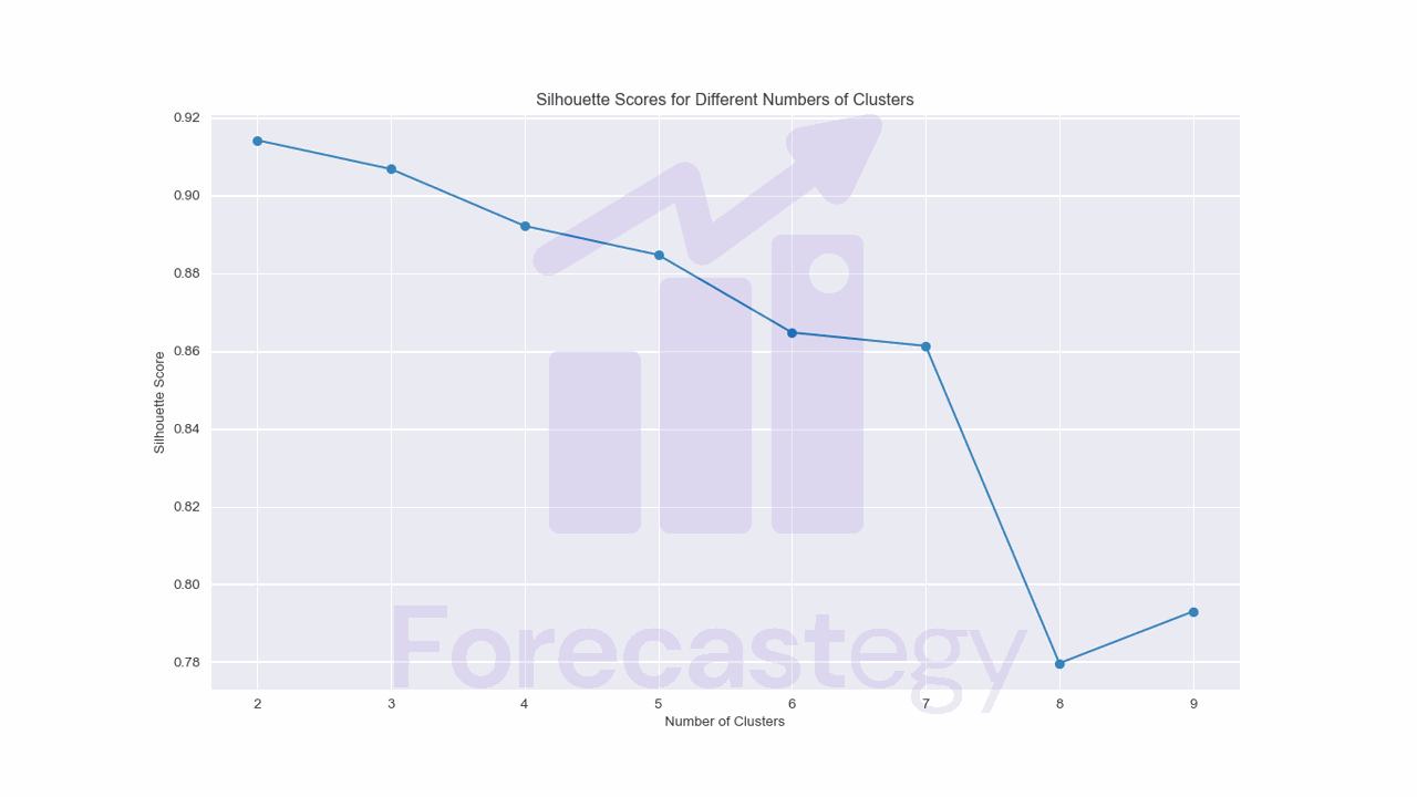
We pass the scaled data and the cluster labels to the silhouette_score function to get the silhouette score for each number of clusters.
Although it says the best number of clusters is 2, I don’t think that’s the case by looking at the data.
So you can use it as a sanity check, but I wouldn’t rely on it too much.
Feature Extraction For Time Series Clustering In Python
Feature extraction can be a powerful technique to transform the raw data into a more manageable format, while capturing relevant information from the time series.
TSFresh is a Python library that automatically extracts up to 1,200 features from time series data.
Some of the features include basic statistics, Fourier and wavelet transforms, and autocorrelation.
To use TSFresh, first install it with pip:
pip install tsfresh
TSFresh can take our data in the original (long) format, where each row represents a single time point and the series are stacked.
from tsfresh import extract_features
from tsfresh.feature_extraction import MinimalFCParameters

df = data[['Date', 'unique_id', 'Sessions']]
extracted_features = extract_features(df, column_id='unique_id', column_sort='Date',
                                      default_fc_parameters=MinimalFCParameters())
Here, we import the extract_features function, which will be used to compute the features for each time series, and the MinimalFCParameters class, which provides a minimal set of feature extraction settings to reduce computation time.
We create a new DataFrame called df containing only the columns needed for feature extraction: 'Date', 'unique_id', and 'Sessions'.
The 'Date' column is the time index, 'unique_id' indicates which rows belong to each individual time series, and 'Sessions' contains the actual time series values.
The extract_features function takes the following arguments:
df: The input DataFrame containing the time series data.column_id: The name of the column that uniquely identifies each time series. In our case, it’s the'unique_id'column, which combines the device category and browser information.column_sort: The name of the column that represents the time index. In our dataset, it’s the'Date'column.default_fc_parameters: The feature set we want to extract. We useMinimalFCParametersto compute a minimal set of features, which reduces the computational complexity and time required for feature extraction. This is a good starting point, but you can experiment with other feature extraction settings provided by tsfresh or create your own custom settings to extract more or different features, depending on your needs and the complexity of your data.
The extract_features function returns a new DataFrame containing the computed features for each time series.
Each row in the DataFrame corresponds to a unique time series, and each column represents a different feature.
| Sessions__sum_values | Sessions__median | Sessions__mean | Sessions__length | Sessions__standard_deviation | Sessions__variance | Sessions__root_mean_square | Sessions__maximum | Sessions__absolute_maximum | Sessions__minimum | |
|---|---|---|---|---|---|---|---|---|---|---|
| desktop_“mozilla | 8456 | 38 | 37.9193 | 223 | 1.12562 | 1.26703 | 37.936 | 40 | 40 | 36 |
| desktop_‘Mozilla | 138889 | 39 | 57.6303 | 2410 | 37.9793 | 1442.43 | 69.0194 | 159 | 159 | 35 |
| desktop_(not set) | 485471 | 37 | 41.1172 | 11807 | 11.5508 | 133.42 | 42.7088 | 80 | 80 | 35 |
| desktop_AdobeAIR | 11546 | 37 | 37.2452 | 310 | 1.46504 | 2.14635 | 37.274 | 40 | 40 | 35 |
| desktop_Bluebeam Revu Browser - cef version: 57.0.0.0 | 15580 | 38 | 38.0929 | 409 | 1.00909 | 1.01826 | 38.1063 | 40 | 40 | 36 |
With the extracted features, you can now proceed with the scaling and clustering steps as we discussed earlier in the tutorial.
from sklearn.cluster import KMeans
from sklearn.preprocessing import StandardScaler

prep = StandardScaler()
kmeans = KMeans(n_clusters=4, random_state=0)

scaled_data = prep.fit_transform(extracted_features)
kmeans.fit(scaled_data)
Now, as we have dense features, we can use StandardScaler to scale the data.
The code is basically the same, but instead of using wide_df, which had the raw time series observations as features, we use extracted_features, which contains the extracted features.
I like this approach because it’s very easy to try different feature extraction methods and compare the results.
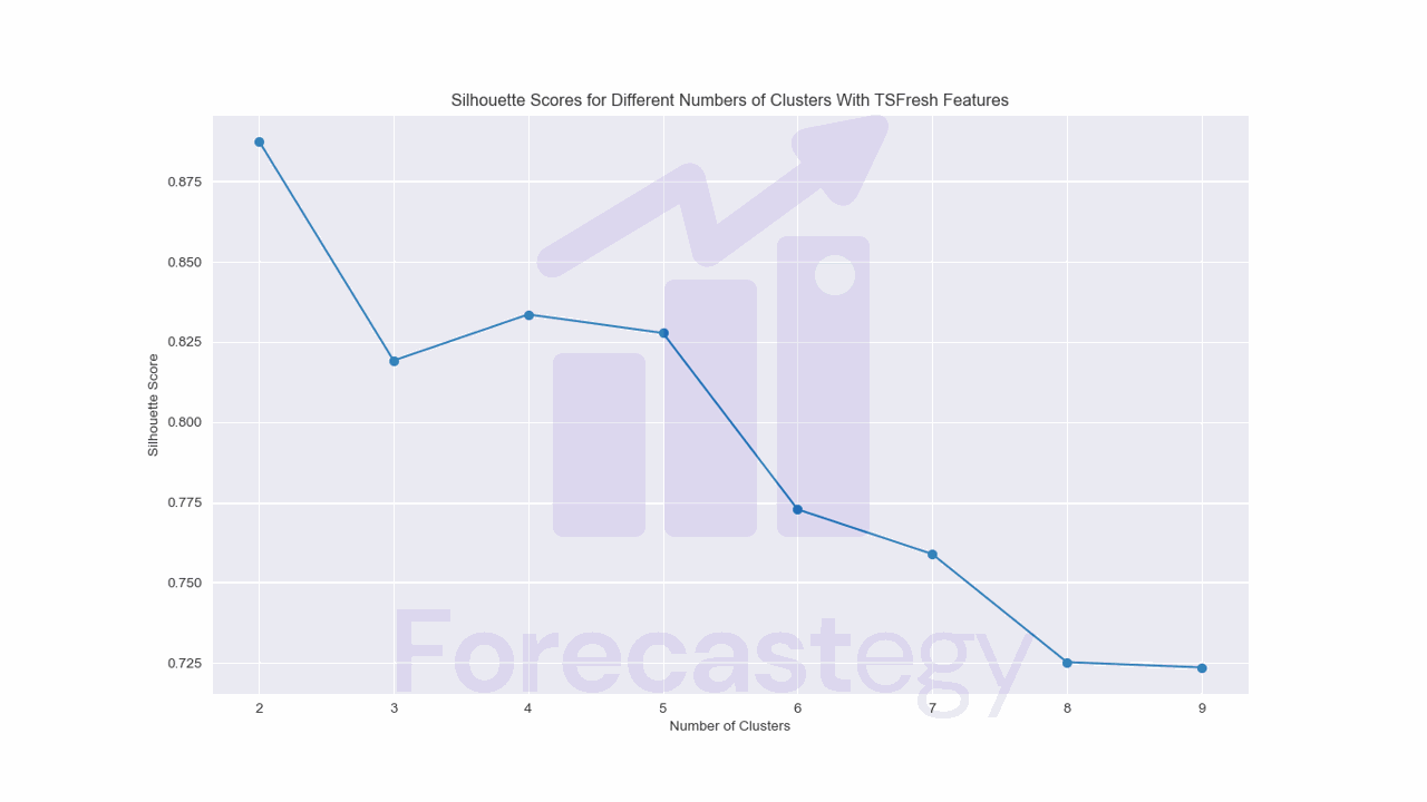
The silhouette score still suggests using only two clusters, but now our clusters changed a bit.
Cluster 0
desktop_"mozilla
desktop_'Mozilla
desktop_(not set)
desktop_AdobeAIR
desktop_Bluebeam Revu Browser - cef version: 57.0.0.0

Cluster 1
desktop_Chrome
mobile_Safari

Cluster 2
desktop_Firefox
desktop_Internet Explorer
desktop_Safari
mobile_Chrome
tablet_Safari

Cluster 3
desktop_Konqueror
Time Series Clustering With PCA Using Scikit-learn
Principal Component Analysis (PCA) is a dimensionality reduction technique that can help you transform your time series data into a lower-dimensional space while preserving the most important information.
It’s another way to do feature extraction.
While feature extraction methods can be domain-specific and interpretable, PCA transforms the data into a new coordinate system, in which the first axis (the first principal component) explains the largest amount of variance in the data, the second axis (the second principal component) explains the second-largest amount of variance, and so on.
It automatically finds the optimal linear projection of the data that preserves the maximum amount of variance.
In practice, I try both approaches and compare the results.
To use PCA for time series clustering, first import the required classes from scikit-learn:
from sklearn.preprocessing import MaxAbsScaler
from sklearn.decomposition import PCA

prep = MaxAbsScaler()
scaled_data = prep.fit_transform(wide_df)

pca = PCA(n_components=2)
pca_data = pca.fit_transform(scaled_data)

kmeans_pca = KMeans(n_clusters=4, random_state=0)
kmeans_pca.fit(pca_data)
We import the MaxAbsScaler class for preprocessing and the PCA class for dimensionality reduction.
As before, we are dealing with the raw time series data first, so we scale using MaxAbsScaler to keep the sparsity.
We create an instance of the PCA class with n_components=2, specifying that we want to reduce the dimensionality of the data to 2 principal components (2 features).
The fit_transform method fits the PCA model to the scaled data (i.e., learns the optimal linear projection) and then transforms the data by projecting it onto the first two principal components.
The transformed data is returned as a new Numpy array called pca_data.
The rest of the code is the same, but applied to the transformed data.
The biggest disadvantage I see is that now we have another hyperparameter to tune: the number of components to keep.
The silhouette score plot now suggests we use between 3 and 4 clusters, which makes more sense for me, looking at the data.
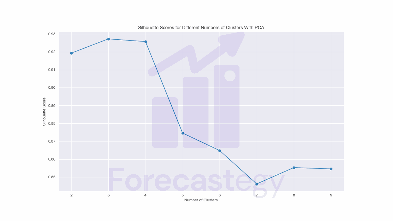
Because of this, mixing my experience and intuition of looking at the examples that got assigned for each cluster, I would consider this approach as the best for clustering this dataset.
Cluster 0
desktop_"mozilla
desktop_'Mozilla
desktop_(not set)
desktop_AdobeAIR
desktop_Bluebeam Revu Browser - cef version: 57.0.0.0

Cluster 1
mobile_Chrome
mobile_Safari

Cluster 2
desktop_Chrome

Cluster 3
desktop_Firefox
desktop_Internet Explorer
desktop_Safari
I love the fact that mobile_Chrome and mobile_Safari are now in the same cluster, which makes sense given that the US tends to have a 50/50 split between Android and iOS users.
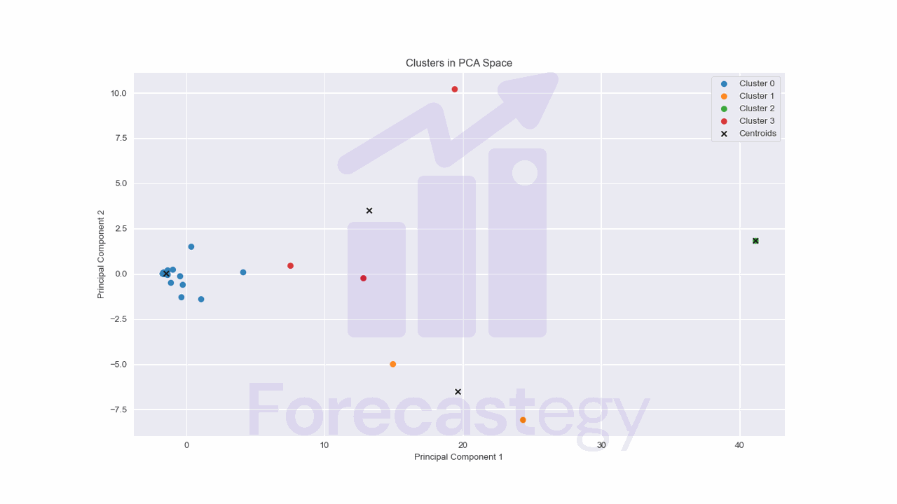
The biggest advantage of using PCA with 2 components is that we can visualize the clusters in a 2D space.
import matplotlib.pyplot as plt

for cluster in range(kmeans_pca.n_clusters):
    cluster_points = pca_data[kmeans_pca.labels_ == cluster]
    plt.scatter(cluster_points[:, 0], cluster_points[:, 1], label=f"Cluster {cluster}")

# Plot the cluster centroids as black 'X' markers
plt.scatter(kmeans_pca.cluster_centers_[:, 0], kmeans_pca.cluster_centers_[:, 1],
            color='black', marker='x', label='Centroids')

plt.title("Clusters in PCA Space")
plt.xlabel("Principal Component 1")
plt.ylabel("Principal Component 2")
plt.legend()

# Display the plot
plt.show()

We have a clear cluster of low activity users, but things get a bit more complicated for the other clusters.