In this article, we will explore the concept of change point detection in time series data using Python.
Change point detection is a powerful technique that helps you identify significant shifts in your time series data, which can provide valuable insights for decision-making and forecasting.
However, detecting change points can be challenging, especially when working with noisy or complex data.
Several algorithms are available, but choosing the right one and fine-tuning its parameters can be time-consuming and confusing.
This is a practical guide on how to apply these algorithms using the Python library Ruptures and real-world data from Google Search Console.
This guide is designed for data analysts, data scientists, and anyone interested in working with time series data.
Let’s get started!
Installing Ruptures
Ruptures is a Python library specifically designed for change point detection.
It provides several algorithms for detecting changes, such as Pelt, Binary Segmentation, and Window-based methods.
You can install ruptures using pip:
pip install ruptures
Preparing The Data For Change Point Detection With Ruptures
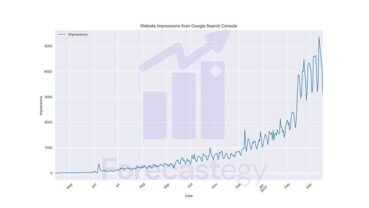
I got data from Google Search Console for this website.
The data contains the number of search impressions for about an year.
This is the number of times a page from this website appeared in Google search results for whatever keywords people were searching for that Google thought were relevant.
import pandas as pd
import numpy as np
import os

data = pd.read_csv(os.path.join(path, 'impressions.csv'), parse_dates=['Date'], usecols=['Date', 'Impressions'])
data.set_index("Date", inplace=True)
data = data.sort_index()

impressions = data["Impressions"].values.reshape(-1, 1)
| Date | Impressions |
|---|---|
| 2022-04-12 00:00:00 | 0 |
| 2022-04-13 00:00:00 | 3 |
| 2022-04-14 00:00:00 | 2 |
| 2022-04-15 00:00:00 | 0 |
| 2022-04-16 00:00:00 | 0 |
As any new website, this one started with zero impressions and slowly grew over time as Google started indexing more pages.
Let’s try all the algorithms available and visually inspect which one works best for our data.
Detecting Change Points With Pelt
PELT (Pruned Exact Linear Time) has a bunch of cool advantages.
One of the top benefits is that it’s super fast when certain conditions are met, making it a great choice for large datasets.
Another perk is that PELT can handle a variety of penalty functions, even the curvy concave ones!
So, it’s pretty versatile and can be used in a range of situations.
However, there are a couple of things to keep in mind.
In some cases, when pruning doesn’t happen, PELT can get a bit slow and end up with a computational cost that grows as the square of the number of data points. So, it’s not always perfect.
Also, when it comes to those curvy concave penalty functions, the simple approach PELT uses to update the penalty constant might not always find the best number of change points.
It can work well sometimes, but in other cases, you might need to use a fancier search method to make sure you get the most accurate results.
Using it with ruptures is pretty straightforward.
import ruptures as rpt

algo = rpt.Pelt(model="l2", min_size=28)
algo.fit(impressions)
result = algo.predict(pen=1)

rpt.display(impressions, [], result)
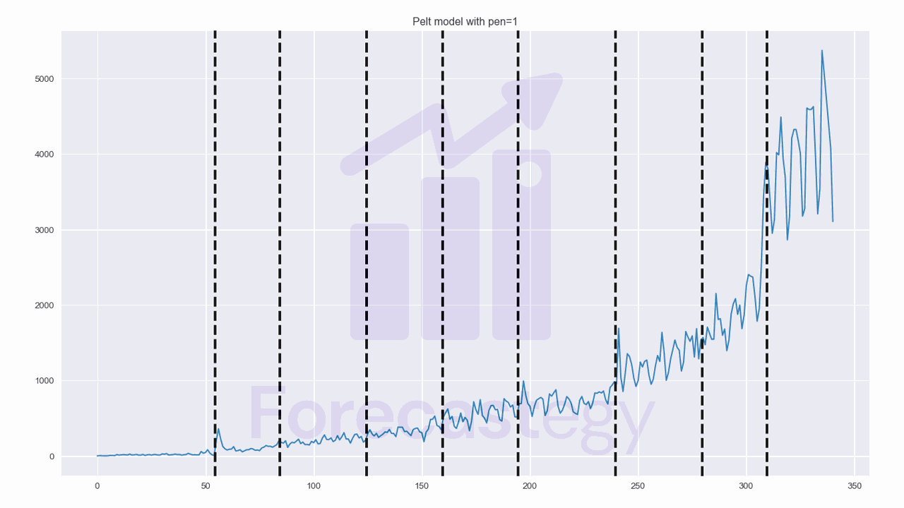
We create an instance of the PELT algorithm using the "l2" model, which is the distance calculated between the time series segments to determine when a change point occurs.
Then we fit the PELT algorithm to the data stored in the impressions variable.
After fitting the algorithm, use the predict method with a specified penalty value (in this case, 1) to get the change points.
I consider these three: model, min_size, and pen as hyperparameters that need to be tuned for each dataset.
The min_size parameter is set to 28, meaning that the minimum length of a segment should be 28 data points.
In other words, the algorithm will not consider change points that are closer than 28 observations.
I selected 28 because changes in search traffic usually happen slowly, with quarter Google updates, for example. So it’s unlikely that a change point will occur within 28 days.
ruptures provides a display function that can be used to visualize the change points detected by the algorithm.
The first argument is the time series data, the second argument is a list of previously known change points, and the third argument is the list of change points detected by the algorithm.
The results seem reasonable for this dataset, but let’s try some other algorithms to see if we can improve it.
Detecting Change Points With Dynamic Programming
DynP leverages a dynamic programming approach to efficiently order the search over all possible segmentations, which helps optimize the process and provide accurate results.
It works by systematically examining all possible segmentations of a given signal to find the exact minimum of the sum of costs associated with each segmentation.
However, one important requirement for using DynP is that the user must specify the number of change points in advance.
While this might be a limitation in certain cases, the method’s flexibility and precision make it a valuable tool for change point detection when the number of change points is known or can be estimated.
The computational complexity of DynP can be another limiting factor, especially when dealing with large datasets or more complex cost functions.
The algorithm may become slow or even impractical for some applications due to its high computational cost.
If you don’t know the number of change points in advance, you can consider it another hyperparameter to tune.
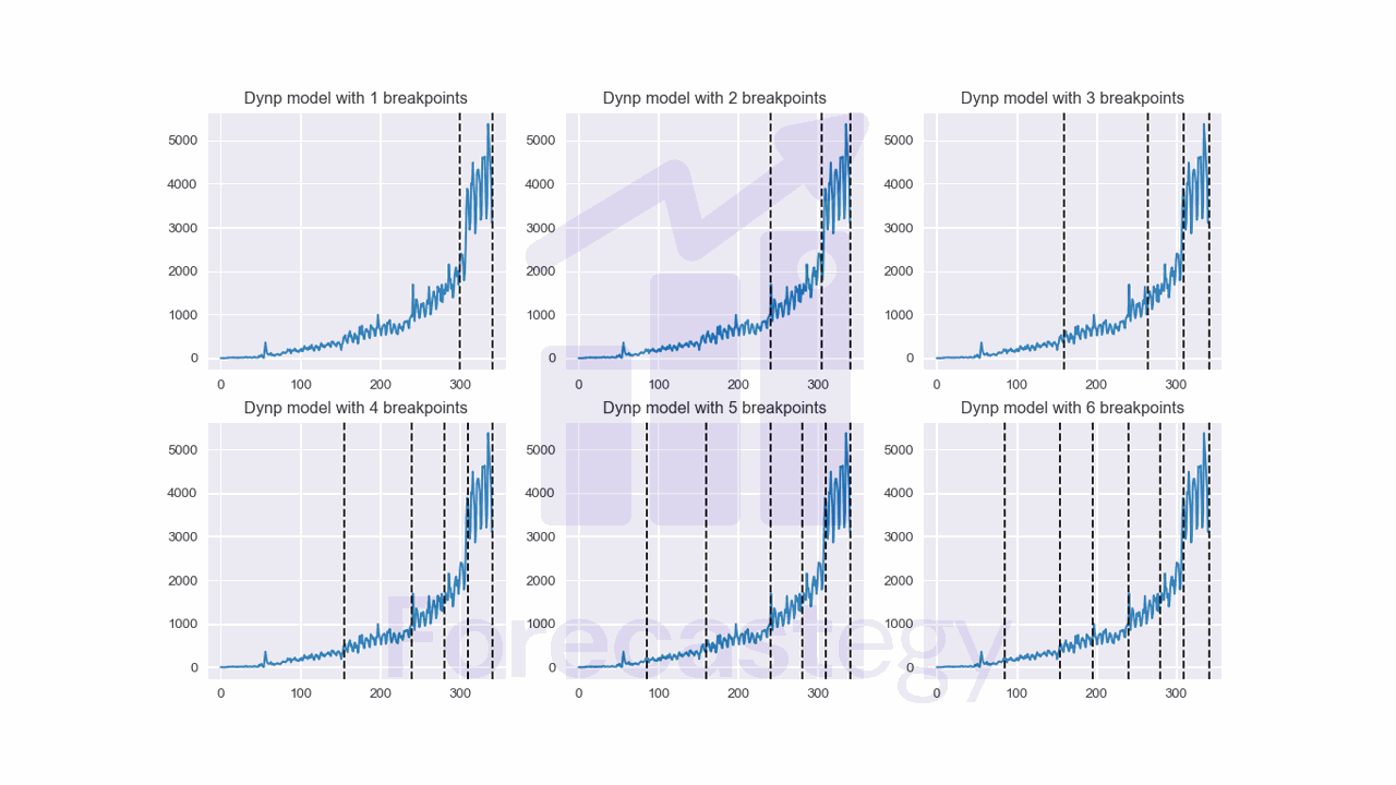
I decided to run a loop to try different values for the number of change points and visually inspect the results to see which one made more sense.
fig, ax = plt.subplots(2,3, figsize=(1280/96, 720/96), dpi=96)
ax = ax.ravel()

algo = rpt.Dynp(model="l2", min_size=28)
algo.fit(impressions)

for i, n_bkps in enumerate([1, 2, 3, 4, 5, 6]):
    result = algo.predict(n_bkps=n_bkps)
    ax[i].plot(impressions)
    for bkp in result:
        ax[i].axvline(x=bkp, color='k', linestyle='--')
    ax[i].set_title(f"Dynp model with {n_bkps} breakpoints")

This code creates a series of subplots displaying the results of the DynP algorithm for change point detection in the impressions time series data.
The algorithm is applied with varying numbers of breakpoints, from 1 to 6, and visualizes the detected change points in each subplot.
I like the results for 5 change points, so I’ll use that value for the rest of the analysis.
Detecting Change Points With Binary Segmentation
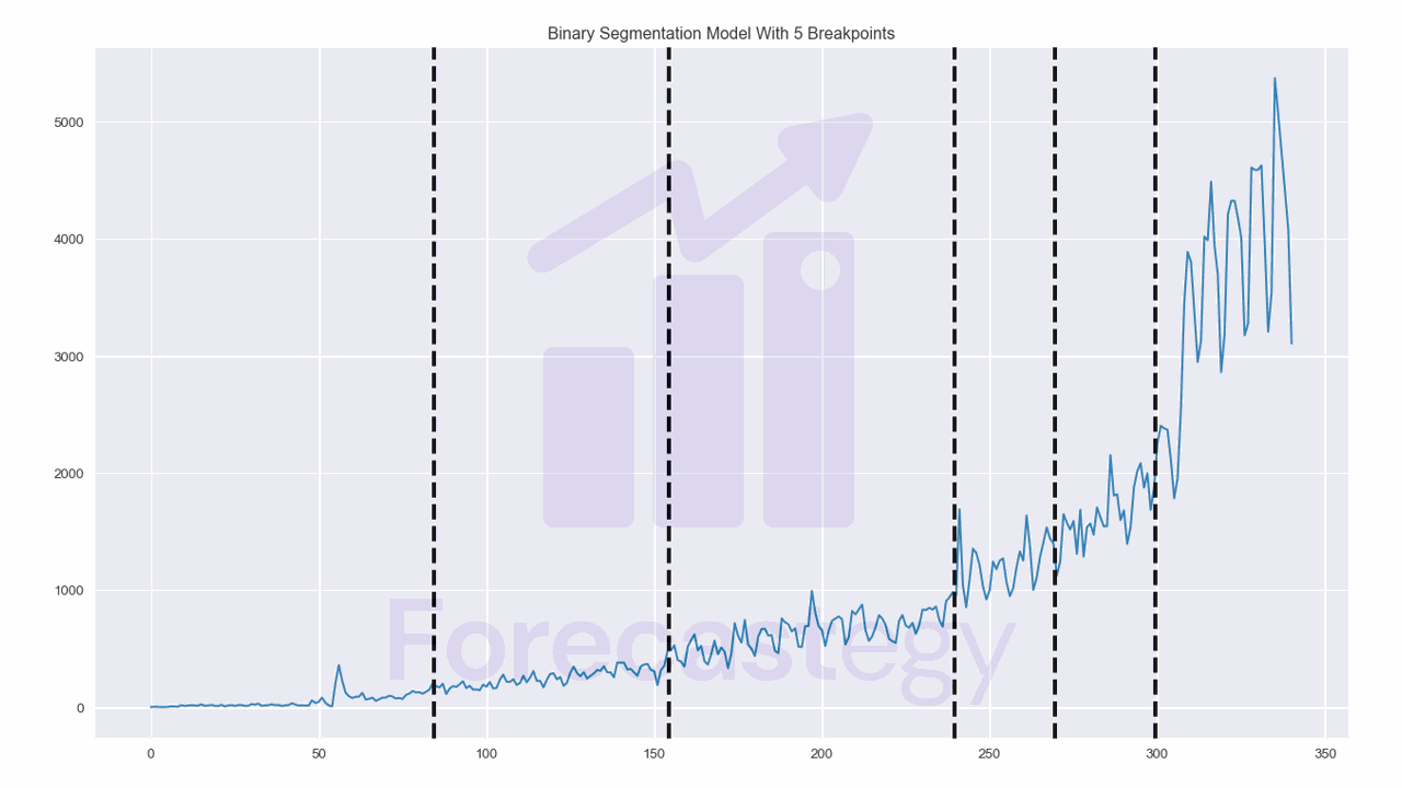
Binary segmentation is pretty simple: first, it looks for a single change point in the entire signal.
Once it finds that point, it splits the signal into two parts and repeats the process for each of those parts.
This keeps going until no more change points are found or a specified stopping criterion is met.
It has a low complexity, which means it doesn’t take too much time or computing power to run and is a good option for large datasets.
One downside is that it can sometimes miss change points or detect false ones, especially when the changes are close together or the signal is noisy.
Additionally, it’s a greedy algorithm, meaning it makes decisions based on the best immediate choice without considering the overall impact on the final result.
This can lead to less-than-optimal solutions in some cases
algo = rpt.Binseg(model="l2", min_size=28)
algo.fit(impressions)
result = algo.predict(n_bkps=5)
Detecting Change Points With Window-Based Method
Window-based change point detection is a pretty nifty method to find where a signal changes.
Imagine two windows sliding along the time series, checking out the properties within each window (like the mean).
What we’re looking for is how similar or different these properties are, and that’s where the discrepancy measure comes in.
Think of the discrepancy as a way to measure how much difference splitting the signal at a certain point would make.
If the properties of the windows are similar, the discrepancy will be low. Else, it will be high, and that’s when we suspect a change point occurred.
One issue is that the choice of window length can have a significant impact on the results.
Too small, and you might miss some change points; too large, and it could ignore important changes.
Instead of using the min_size parameter, we can use the width parameter to specify the window length.
algo = rpt.Window(model="l2", width=28)
algo.fit(impressions)
result = algo.predict(n_bkps=5)
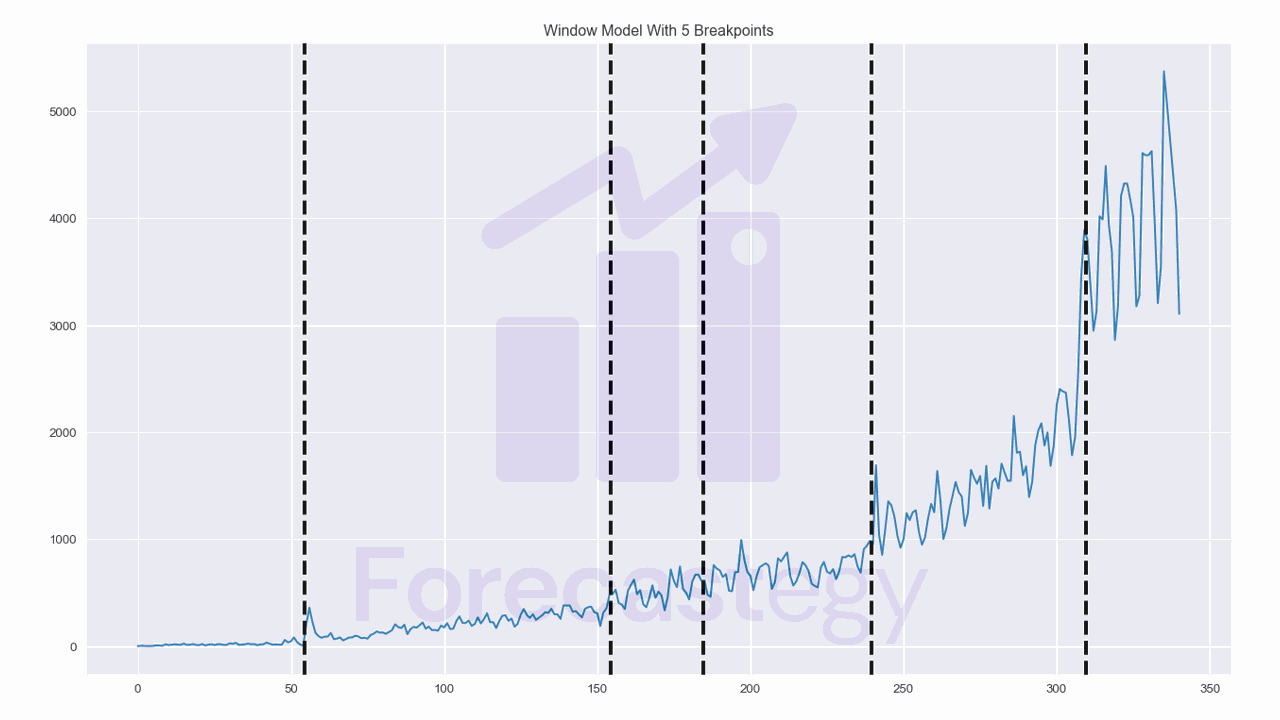
The results look good!
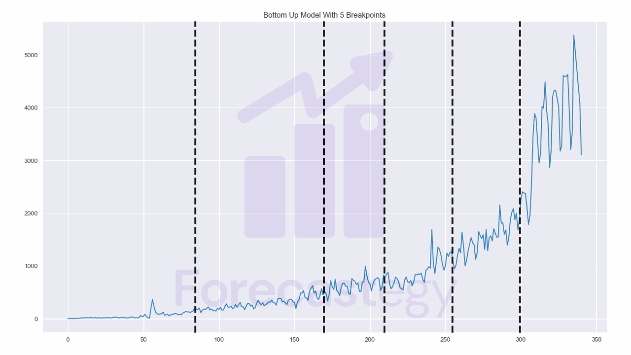
Detecting Change Points With The Bottom-Up Method
Bottom-up segmentation is an interesting approach for detecting change points in a signal.
Instead of starting with a single segment and dividing it, bottom-up segmentation begins with numerous change points and gradually reduces them.
Think of it like assembling a massive puzzle and then removing the pieces that don’t quite belong.
Here’s how it goes: first, the signal is split into smaller pieces along a regular pattern.
Then, these pieces are progressively combined based on their similarities.
If two adjacent segments are alike, they’re joined into one larger segment.
This process continues until we’re left with the most meaningful change points
algo = rpt.BottomUp(model="l2", min_size=28)
algo.fit(impressions)
result = algo.predict(n_bkps=5)
Detecting Change Points With Kernel Change Detection
Kernel change point detection works by mapping the signal to a higher-dimensional space, called a Reproducing Kernel Hilbert Space (RKHS).
This might sound fancy, but it’s just a way to make change point detection more powerful and versatile by analyzing the signal from a different perspective.
The core idea is to find the change points that minimize a certain cost function, which measures how well the segmented signal fits the data.
When the number of change points is known, you can solve a specific optimization problem to find the best segmentation.
If you don’t know the number of change points, you can use a penalty term to balance the goodness of fit against the complexity of the segmentation.
There are three kernel functions available in ruptures: Linear, RBF, and Cosine.
Each of these kernels offers a different way to analyze the signal, giving you the flexibility to choose the most suitable approach for your data.
I decided to run a loop to try different values for the kernels and visually inspect the results again to see which one made more sense.
fig, ax = plt.subplots(3,1, figsize=(1280/96, 720/96), dpi=96)

for i, kernel in enumerate(['linear', 'rbf', 'cosine']):
    algo = rpt.KernelCPD(kernel=kernel, min_size=28)
    algo.fit(impressions)
    result = algo.predict(n_bkps=5)
    ax[i].plot(impressions)
    for bkp in result:
        ax[i].axvline(x=bkp, color='k', linestyle='--')
    ax[i].set_title(f"Kernel model with {kernel} kernel")
fig.tight_layout()
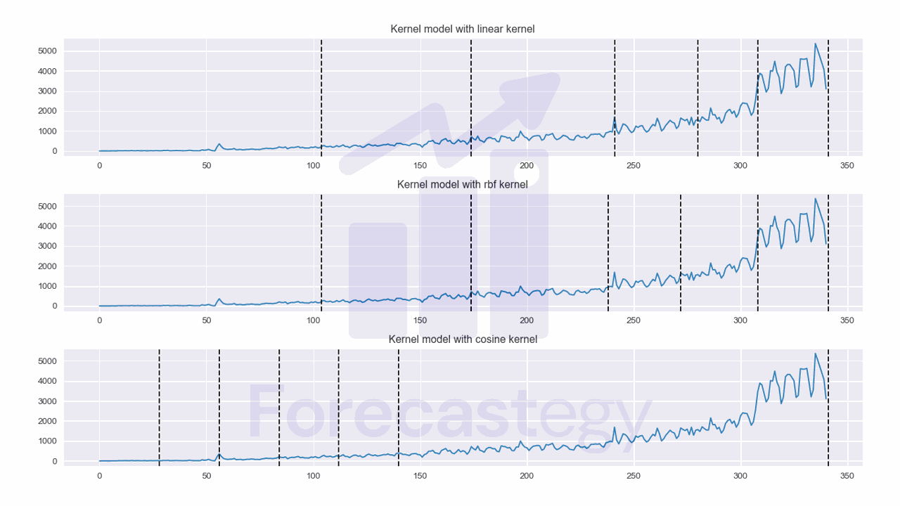
I really liked the results for the RBF kernel.
See how the cosine kernel gave bad results? That’s why it’s important to try different kernels.