In this blog post, we will explore how we can use Python to forecast volatility using three methods: Naive, the popular GARCH and machine learning with scikit-learn.
Volatility here is the standard deviation of the returns of a financial instrument.
I will teach you starting points to kickstart your own research.
Installing ARCH and mlforecast
First we need to install the required packages. You can do it with pip:
pip install arch
pip install mlforecast
or with conda:
conda install -c conda-forge arch-py
conda install -c conda-forge mlforecast
With Arch we will use the GARCH model and with mlforecast we will use a Scikit-learn model.
Preparing The Data For Volatility Forecasting
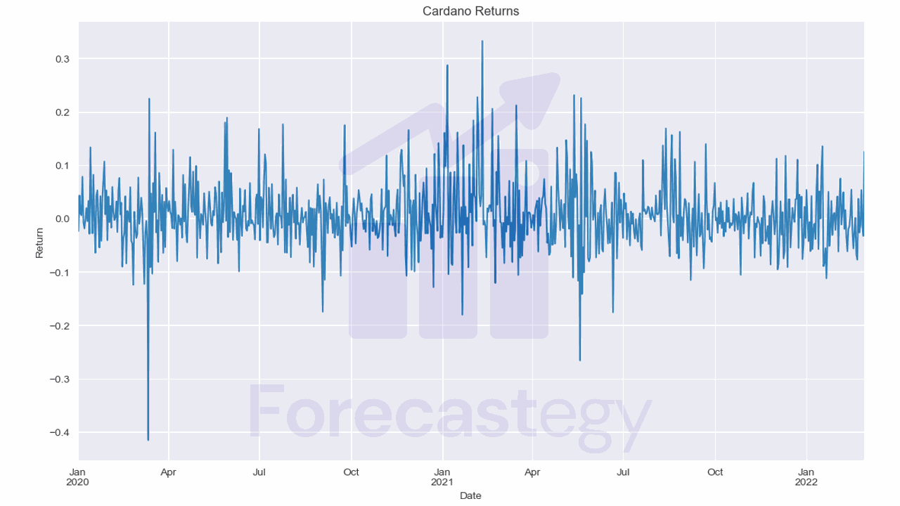
We will use real crypto data available at Kaggle.
This tutorial is applicable to any financial instrument, I just got crypto because it was easily available.
I took only 20 coins to run faster, but you can use all of them.
import pandas as pd
import glob

data = list()
for f in glob.glob(path)[:20]:
    fname_noext = f.split(os.sep)[-1].split(".")[0]
    data_ = pd.read_csv(f, parse_dates=['Date'])
    data_['coin'] = fname_noext
    data_['return'] = data_['Close'].pct_change()
    data_['target_realized_vol'] = data_['return'].rolling(7).std().shift(-7)
    data_ = data_[data_['Date'] >= '2020-01-01']
    data.append(data_)
data = pd.concat(data, axis=0, ignore_index=True)
Each file contains the historical data of a coin.
Our target is the target_realized_vol column, which is the standard deviation of the returns of the next 7 days for each coin.
Some coins have a long history, others don’t, the cutoff date at 2020-01-01 is arbitrary.
We need to split the data into train and validation sets. I picked 2022-03-01 as the split date.
split = "2022-03-01"
train  = data[data['Date'] < split]
valid = data[data['Date'] >= split]
coins = valid['coin'].unique()
We need to be very careful with the training data here, as we created the target column before doing the split.
I will explain why in the next section.
Some people like to split the data by coin instead of by time, but I really don’t like it in a scenario with lots of highly correlated data like the one here.
Naive Volatility Forecasting
First up, let’s talk about the Naive method.
This method is simple and intuitive, making it a great starting point for understanding volatility forecasting.
The Naive method assumes that the volatility of a financial instrument over a given period is equal to the volatility observed during the previous period.
It is called “Naive” because it’s a simple rule that does not take into account any other factors that might influence volatility.
Here we will take the last target value and use it as the prediction for the next period.
from sklearn.metrics import mean_squared_error

p = train[train['Date'] == '2022-02-21'][['Date', 'coin','target_realized_vol']]
p = p.rename(columns={'target_realized_vol':'pred'})
p['Date'] = p['Date'] + pd.DateOffset(8)
p = p.merge(valid[['Date', 'coin','target_realized_vol']], on=['Date', 'coin'], how='left')

mean_squared_error(p['target_realized_vol'], p['pred'], squared=False)
| Date | coin | pred | target_realized_vol |
|---|---|---|---|
| 2022-03-01 00:00:00 | 1inch | 0.0546111 | 0.028911 |
| 2022-03-01 00:00:00 | Aave | 0.0692836 | 0.0379977 |
| 2022-03-01 00:00:00 | Algorand | 0.0566661 | 0.0249555 |
| 2022-03-01 00:00:00 | ApeCoin | 0.0539567 | 0.0368307 |
| 2022-03-01 00:00:00 | Arweave | 0.0569066 | 0.0657768 |
Pay attention to the Date I selected.
We are pretending to make a prediction on February 28, 2022.
Our training data goes until February 28, 2022, but in practice we don’t know the target for the last 7 days of our data, as these include days that are in the validation set.
Think about it, the target for February 26, 2022 is the standard deviation of the returns of the next 7 days, which ends on March 5, 2022.
Taking the target value from any date after February 21, 2022 would introduce data leakage.
With that in mind, I got the values for each coin and shifted the date in the rows to 8 days after (March 1, 2022), which is the day we want to predict.
Then I merged the predictions with the validation set and calculated the RMSE, which was 0.0244.
Naive baselines tend to be strong and hard to beat in financial time series forecasting, so let’s see if the more complex models can do better.
GARCH For Volatility Forecasting
GARCH, which stands for Generalized Autoregressive Conditional Heteroskedasticity, is a more advanced approach to volatility forecasting, and it takes into account the fact that volatility tends to cluster together over time.
This means that when we observe high volatility today, it is more likely that we will also observe high volatility tomorrow.
GARCH models use traditional statistical modeling to estimate how volatility changes over time, and they are widely used in finance.
Disclaimer: I am approaching this topic with the eyes of a machine learning engineer, not a statistician. Someone with more experience with GARCH may get different results.
We need a loop to run the model for each coin, as the library doesn’t support multiple time series at once.
from arch import arch_model

results = list()
for coin in coins:
    returns = train[train['coin'] == coin]['return'].dropna().clip(-1,1)

    am = arch_model(returns, vol="Garch", p=1, q=1)
    res = am.fit()
    p = np.sqrt(res.forecast(reindex=False, horizon=7).variance).mean(axis=1)
    y = valid[valid['coin'] == coin]['target_realized_vol'].iloc[0]

    results.append({'coin': coin, 'predicted': p.values[0], 'realized': y})

df = pd.DataFrame(results).sort_values('realized', ascending=False)
print(mean_squared_error(df['realized'], df['predicted'], squared=False))
| coin | predicted | realized |
|---|---|---|
| Celo | 0.136376 | 0.0684473 |
| Arweave | 0.0901401 | 0.0657768 |
| Basic Attention Token | 0.0688667 | 0.041834 |
| chainlink | 0.0723431 | 0.0403548 |
| Axie Infinity | 0.0820315 | 0.0395899 |
For each coin we take the returns from the training set, clipped to be between -1 and 1.
The function arch_model creates the model. The first argument is the series of returns.
We can pass the full series because we are assuming a prediction on February 28, 2022 at the end of the day. So we have all the returns up to and including this date.
The second argument is the type of model we want to use to model the volatility.
The p and q arguments are the order of the autoregressive and moving average terms, respectively.
It basically means how many previous values we want to use to predict the next one.
I consider these as hyperparameters that you can tune for each coin or for all of them at once.
After fitting the model we get the volatility forecast by calling the forecast method and getting the variance attribute.
Here I put horizon=7 because we want to predict the volatility for the next 7 days.
As I am not completely sure about the time duration of GARCH forecasts, I just averaged the values.
Again, I am looking here for something that works, not for the rigorous statistical approach.
The variance is the square of the standard deviation, so I took the square root to get the standard deviation which is what our target is.
The RMSE was 0.0382, which is worse than the naive baseline.
Volatility Forecasting With Scikit-Learn
We can use any scikit-learn model or even XGBoost to predict volatility easily by using the mlforecast library.
First we need to prepare the data with the same care we did for the Naive model.
train_ml = train.groupby('coin', as_index=False).apply(lambda x: x.iloc[:-7]).reset_index(drop=True)
train_ml = train_ml.rename(columns={'Date': 'ds', 'target_realized_vol': 'y', 'coin': 'unique_id'})[['ds', 'unique_id', 'y']]
valid_ml = valid.rename(columns={'Date': 'ds', 'target_realized_vol': 'y', 'coin': 'unique_id'})[['ds', 'unique_id', 'y']]
Here we remove the last 7 days from the training set, as we don’t know the target for these days.
Then we rename the columns to match the mlforecast library requirements.
dsis the date columnunique_idis the column that identifies the time series (each coin)yis the target column
Let’s create a Random Forest model and fit it to the data.
from mlforecast import MLForecast
from window_ops.rolling import rolling_mean, rolling_std
from sklearn.ensemble import RandomForestRegressor

model = MLForecast(models=[RandomForestRegressor(random_state=0, n_jobs=-1)],
                   freq='D',
                   lags=[1,3,7,14],
                   lag_transforms={1: [(rolling_mean, 3), (rolling_mean, 7)]})
model.fit(train_ml, id_col='unique_id', time_col='ds', target_col='y', static_features=[])
We import the MLForecast class from the mlforecast library.
Then we create a list of models to use. In this case, we only have one model, but you can pass a list of models and the library will train all.
The freq argument is the frequency of the time series. In our case, it is daily.
The lags argument is a list of lags to use. In this case, we use 1, 3, 7 and 14 days. You can try different values and see how they affect the results.
The lag_transforms argument is a dictionary that maps the lag to a list of more complex transformations to apply to the lag.
For example, we will apply a rolling mean with a window of 3 and 7 days to the lag of 1 day.
This means the library will take the original series, shift it by 1 day, and then apply the rolling mean.
To do it for other lags you just have to add the number as a key and the list of transformations as the value.
Note that we pass a list of tuples, where the first element is the function and the second is the window.
If we had more arguments, we could just pass them as additional items in the tuple.
Here we use functions from the window_ops library, which is optimized. The developers of MLForecast recommend using it and numba if you want to use custom functions.
We need to specify the columns related to the date, the unique id and the target in the fit method.
Besides, we can pass a list of static features (e.g: the exchange where the data was taken from). I like to pass an empty list here because if we decided to add external features, they will be treated as static unless we specify which columns are really static.
The prediction is straightforward.
p = model.predict(horizon=8)
p = p.merge(valid_ml, on=['ds', 'unique_id'], how='left').dropna()
mean_squared_error(p['y'], p['RandomForestRegressor'], squared=False)
The predict method returns a dataframe with the predictions for each coin and each day in the horizon.
| unique_id | ds | RandomForestRegressor | y |
|---|---|---|---|
| 1inch | 2022-03-01 00:00:00 | 0.0406654 | 0.028911 |
| Aave | 2022-03-01 00:00:00 | 0.0415011 | 0.0379977 |
| Algorand | 2022-03-01 00:00:00 | 0.0425734 | 0.0249555 |
| ApeCoin | 2022-03-01 00:00:00 | 0.0455959 | 0.0368307 |
| Arweave | 2022-03-01 00:00:00 | 0.0401673 | 0.0657768 |
The horizon is the number of days to predict after the last date in the training set.
As we have a gap of 7 days between the training and validation sets, we need to predict 8 days.
Then we merge the predictions with the validation set and calculate the RMSE.
The RMSE was 0.0224, which is slightly better than the naive baseline.
This model can be improved by adding more features, tuning the hyperparameters.
It’s a good idea to extend the validation and calculate the RMSE for more days than just a single one like I did here to demonstrate.