
In machine learning, we often come across datasets where the number of observations in one class significantly outweighs the other.
This is known as imbalanced data.
For instance, in a dataset of credit card transactions, the number of fraudulent transactions (positive class) is usually much smaller than the number of legitimate transactions (negative class).
This is also an example of a binary classification task, which is a common type of machine learning problem.
When dealing with imbalanced data in binary classification, the model can become biased toward the majority class, leading to poor performance on the minority class.
If you have 1 fraudulent transaction and 99 legitimate transactions, a model that always predicts the transaction to be legitimate will have an accuracy of 99%.
However, this model is useless because it never predicts a fraudulent transaction, which is the one we’re interested in.
XGBoost is a powerful gradient-boosting library that offers us a simple way to handle imbalanced data.
Don’t be fooled by the simplicity of this approach: in my experience, it was NEVER outperformed by more complex methods like SMOTE.
Trust me, I tried a lot of them.
As a bonus, you can use this approach for multiclass classification as well.
Keep reading to learn how to use this powerful approach to handle imbalanced data in your XGBoost models.
Loading The Imbalanced Dataset
Let’s start by loading the Red Wine Quality dataset from UCI.
This is a popular dataset that we will use throughout this tutorial.
It contains 11 features measuring different chemical properties of red wine, and the target variable is the quality of the wine, which is a score between 3 and 8.
It doesn’t have any categorical variables, so we don’t need to worry about encoding them.
We will binarize the target variable to create a binary classification task.
Every wine with a quality score of 7 or higher will be assigned a value of 1, and the rest will be assigned a value of 0.
First, we need to import the necessary libraries and load the dataset:
import pandas as pd
from sklearn.model_selection import train_test_split

# Load the dataset
url = "https://archive.ics.uci.edu/ml/machine-learning-databases/wine-quality/winequality-red.csv"
data = pd.read_csv(url, sep=";")

# Binarize the target variable
data['quality'] = [1 if x >= 7 else 0 for x in data['quality']]
Next, let’s split the data into training and test sets:
# Split the data into training and test sets
X = data.drop('quality', axis=1)
y = data['quality']
X_train, X_test, y_train, y_test = train_test_split(X, y, test_size=0.2, random_state=42)
Now, let’s check the class distribution in our training set:
# Check class distribution
y_train.value_counts()

0    1109
1     170
You’ll notice that the number of observations in one class is significantly higher than in the other, indicating that we have an imbalanced dataset.
My rule of thumb is to start worrying about imbalanced data when at least 80% of the observations are in one class.
In this case, we have 87.5% of the observations in one class, so we need to handle this imbalance.
Using scale_pos_weight (Class Weight) To Handle Imbalanced Data
When dealing with imbalanced data, one common approach is to assign a higher penalty to misclassifications of the minority class.
This can be achieved using the scale_pos_weight parameter in XGBoost.
Think about the scale_pos_weight value as a multiplier for the loss function evaluated on the positive class.
By default, it’s set to 1, meaning that both classes have the same weight.
If we set it to a value greater than 1, the model will give more importance to the positive class, as it will be penalized more for misclassifying this class.
The suggested way to set the scale_pos_weight value is by dividing the number of negative samples by the number of positive ones.
Let’s calculate this ratio for our training set:
# Calculate the ratio of negative class to positive class
ratio = float(y_train.value_counts()[0]) / y_train.value_counts()[1]
Now, we can use this ratio as the scale_pos_weight value when training our XGBoost model.
In this case, every positive sample mistake the model makes will cost 6.52 times a negative sample mistake.
This will help the model pay more attention to the minority class during training, potentially improving its performance in this class.
Like I said before, although simple, it’s the most powerful approach I’ve ever used to handle imbalanced data in any machine learning model.
I even asked experienced colleagues about it, and they had the same experience.
In the next section, we’ll train an XGBoost model using this scale_pos_weight value.
Training XGBoost Classifier With scale_pos_weight
First, we need to import the XGBoost library:
import xgboost as xgb
Next, we’ll create an instance of the XGBoost classifier, passing in our scale_pos_weight value:
# Create an XGBoost classifier with the scale_pos_weight value
model = xgb.XGBClassifier(scale_pos_weight=ratio)
Now, we can fit the model to our training data:
# Fit the model to the training data
model.fit(X_train, y_train)
And that’s everything you need to do!
We’ve trained an XGBoost model on imbalanced data, using the scale_pos_weight parameter to give more importance to the minority class.
Let’s see how it performs on the test set.
Evaluating The Model
After training our model, it’s important to evaluate its performance.
We’ll use two metrics for this: ROC-AUC (Area Under the ROC Curve), and F1 score.
You might be asking: why not log loss?
I don’t like log loss when using different weights for the classes, as it’s not adequate for the problem: if you need calibrated probabilities, it makes no sense to push the model to predict the minority class more often, which is what the scale_pos_weight parameter does.
ROC AUC is a common evaluation metric for binary classification problems.
It measures the ability of the classifier to rank observations from the positive class higher than observations from the negative class.
A perfect classifier will have an ROC AUC score of 1, while a random classifier will have an ROC AUC score of 0.5.
The F1 score is the harmonic mean of precision and recall. It’s a good metric to use when the classes are imbalanced.
I don’t like to optimize the F1 Score directly, as we need to define a threshold to convert the predicted scores into class labels before calculating it.
I recommend you develop your model optimizing the ROC AUC score on the validation set, and after maximizing it, you can choose the threshold that maximizes the F1 score.
Let’s see how to calculate these metrics for our model.
First, we need to import the necessary functions from sklearn.metrics:
from sklearn.metrics import roc_auc_score, f1_score
Next, we’ll make predictions on the test set and calculate the metrics:
# Make predictions on the test set
y_pred = model.predict(X_test)
y_pred_proba = model.predict_proba(X_test)[:, 1]

# Calculate AUC
auc = roc_auc_score(y_test, y_pred_proba)
print(f"AUC: {auc}")

# Calculate F1 score
f1 = f1_score(y_test, y_pred)
print(f"F1 Score: {f1}")
model.predict(X_test) returns the predicted class labels with a threshold of 0.5, while model.predict_proba(X_test) returns the predicted probabilities.
As you can see, we take only the column corresponding to the positive class when calculating the ROC AUC score.
Remember, the goal is not just to maximize the accuracy, but also to ensure that the model performs well on the minority class, which is often the class of interest in imbalanced datasets.
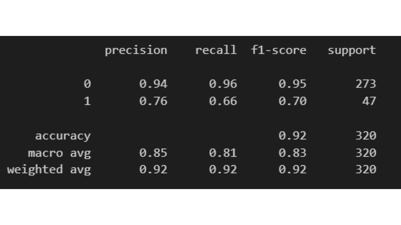
Another very useful function from scikit-learn is classification_report, which gives us a summary of the most important classification metrics:
from sklearn.metrics import classification_report
print(classification_report(y_test, y_pred))
Just like any other hyperparameter, to optimize the threshold to maximize the F1 score, we can use a simple for loop:
for th in range(1,11,1):
    th = th / 10
    y_pred = (y_pred_proba > th).astype(int)
    f1 = f1_score(y_test, y_pred)
    print(f"Threshold: {th} - F1: {f1}")
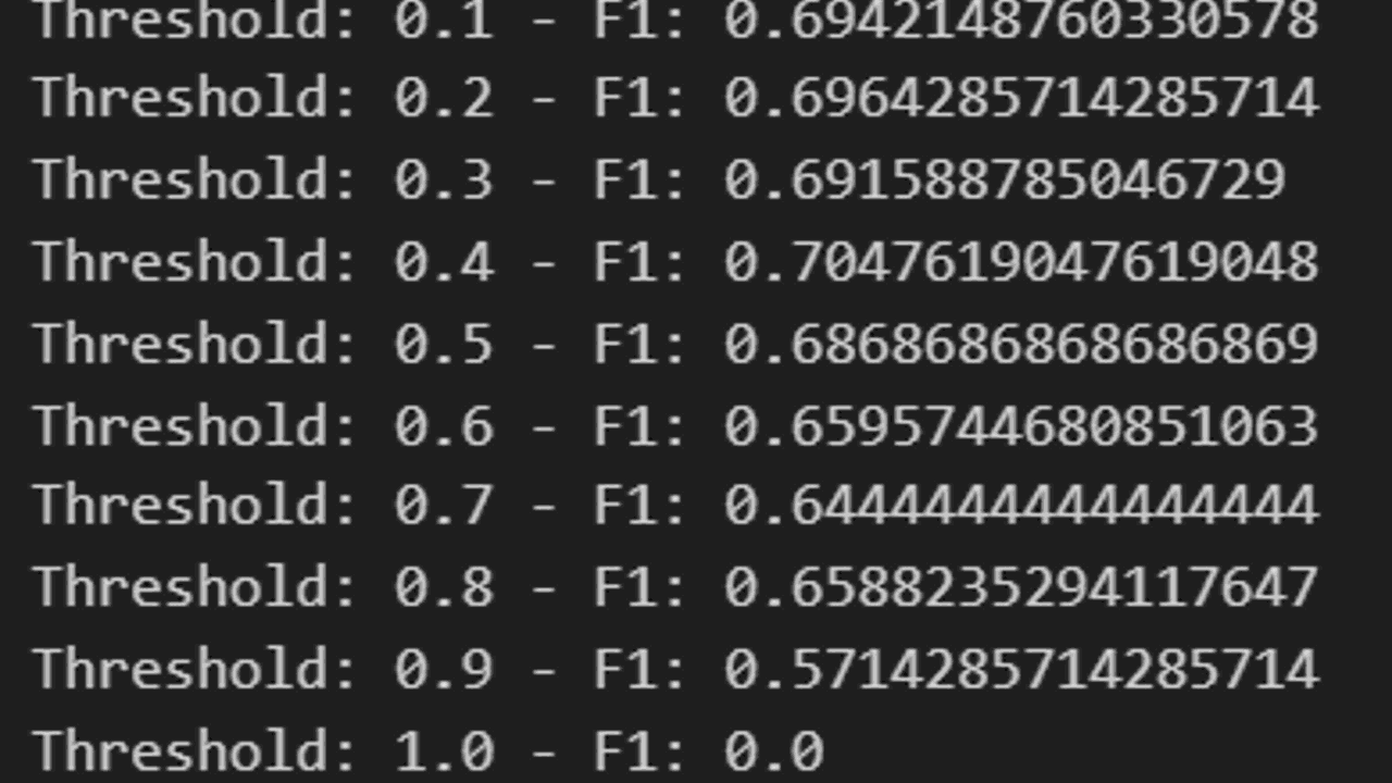
Here we iterate over a range of values from 0.1 to 1, and for each value, we convert the predicted probabilities into class labels using that threshold.
Then, we calculate the F1 score for the predicted labels and print it.
You can do the same for other thresholded metrics like precision and recall, and choose the threshold that maximizes the metric you’re most interested in.
Just don’t go too crazy on the granularity of the range, as it can overfit the test set.