When working with time series data, differencing is a common technique used to make the data stationary.
Stationary data is important because it allows us to apply statistical models that assume constant parameters (like the mean and standard deviation) over time, and this can improve the accuracy of our predictions.
Let’s see how we can easily perform differencing in Python using Pandas, Numpy, and Polars.
First-order Differencing
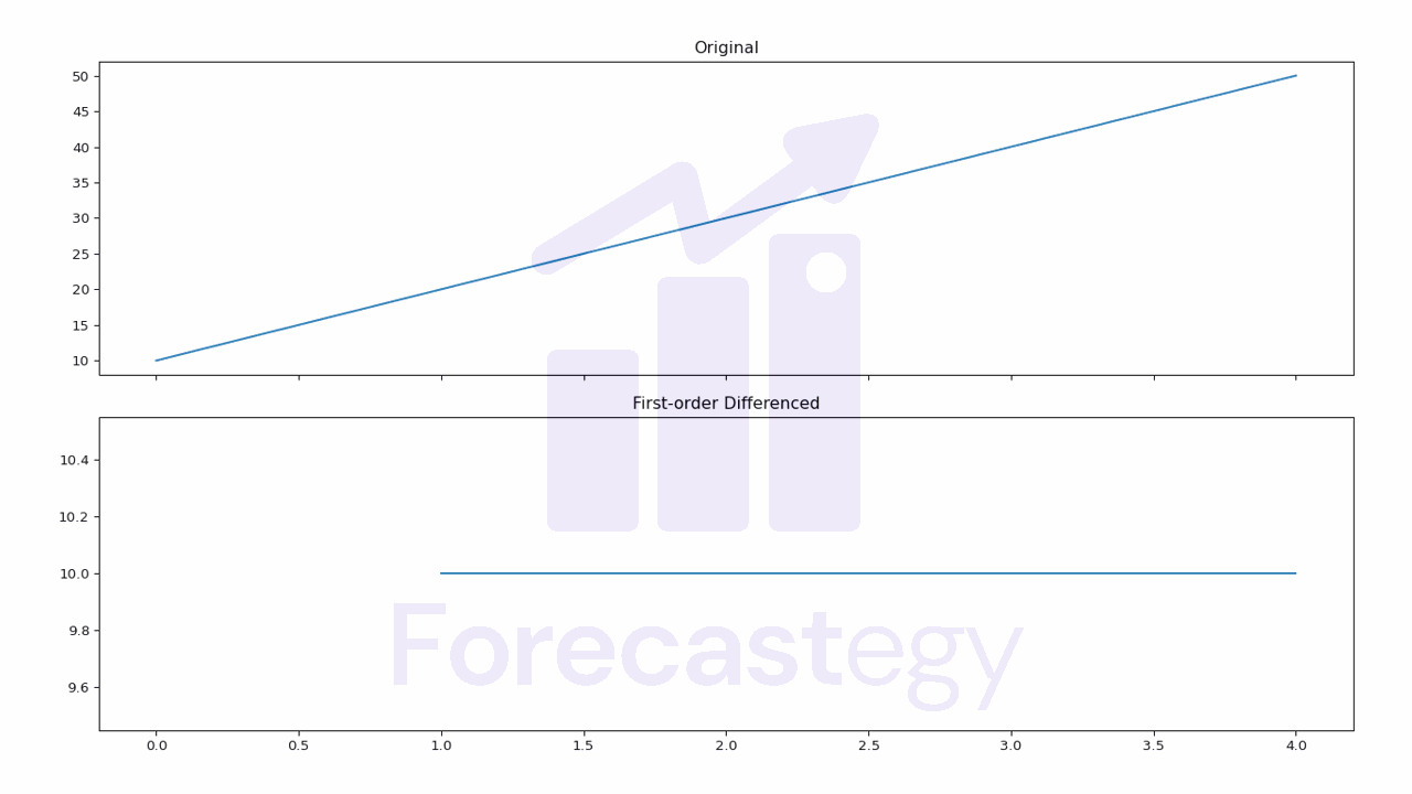
First-order differencing involves subtracting each value in the time series from its previous value.
Pandas
In Pandas, we can perform first-order differencing using the diff() method. Here’s an example:
import pandas as pd

ts = pd.Series([10, 20, 30, 40, 50])

ts_diff = ts.diff()

print(ts_diff)

| diff | |
|---|---|
| 0 | nan |
| 1 | 10 |
| 2 | 10 |
| 3 | 10 |
| 4 | 10 |
Note that the first value is NaN because there is no previous value to subtract from.
Notice the y-axis values in the plot to see the difference.
Numpy
In Numpy, we can perform first-order differencing using the np.diff() function.
import numpy as np

ts = np.array([10, 20, 30, 40, 50])

ts_diff = np.diff(ts)

print(ts_diff)

#output
[10 10 10 10]
This time the first value is removed.
Polars
In Polars, we can perform first-order differencing using the shift() method.
import polars as pl

ts = pl.Series([10, 20, 30, 40, 50])

ts_diff = ts.diff()

print(ts_diff)

# output
shape: (5,)
Series: '' [i64]
[
	null
	10
	10
	10
	10
]
Again, the first value is null because there is no previous value to subtract from.
Second-order Differencing
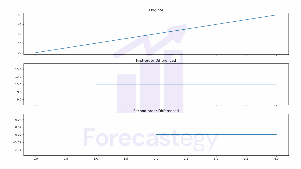
Second-order differencing involves taking the simple difference of values on a time series twice.
This can be useful in some cases where a first-order difference is not enough to make the time series stationary.
Pandas
In Pandas, we can perform second-order differencing by calling the diff() method twice.
import pandas as pd

ts = pd.Series([10, 20, 30, 40, 50])

ts_diff = ts.diff().diff()

print(ts_diff)
| diff_diff | |
|---|---|
| 0 | nan |
| 1 | nan |
| 2 | 0 |
| 3 | 0 |
| 4 | 0 |
Now our first and second values are NaNs.
Notice the y-axis values in the plot to see the difference.
Numpy
In Numpy, we can perform second-order differencing by calling the np.diff() function twice.
import numpy as np

ts = np.array([10, 20, 30, 40, 50])

ts_diff = np.diff(np.diff(ts))

print(ts_diff)

# output
[0 0 0]
Polars
In Polars, we can perform second-order differencing by calling the shift() method twice.
import polars as pl

ts = pl.Series([10, 20, 30, 40, 50])

ts_diff = ts.diff().diff()

print(ts_diff)

## output
shape: (5,)
Series: '' [i64]
[
	null
	null
	0
	0
	0
]
Basically the same as Pandas.
Seasonal Differencing
Seasonal differencing involves subtracting the value of a time series from the value at the same time in the previous season.
This can be useful in cases where the time series exhibits a seasonal pattern.
For example, if we have a time series of monthly sales data, we would subtract the value of the same month in the previous year from the current month.
If we have a time series of daily sales data, we could subtract the value of the same day in the previous week from the current day.
Pandas
In Pandas, we can perform seasonal differencing by calling the diff() method with the appropriate lag.
import pandas as pd

dates = pd.date_range(start='2021-12', end='2023-12', freq='M')
ts = pd.Series([10, 20, 30, 40, 50, 10, 20, 30, 40, 50, 10, 20] * 2, index=dates)

ts_diff = ts.diff(periods=12)

print(ts_diff)
| ts | ts_diff | |
|---|---|---|
| 2021-12-31 00:00:00 | 10 | nan |
| 2022-01-31 00:00:00 | 20 | nan |
| 2022-02-28 00:00:00 | 30 | nan |
| 2022-03-31 00:00:00 | 40 | nan |
| 2022-04-30 00:00:00 | 50 | nan |
| 2022-05-31 00:00:00 | 10 | nan |
| 2022-06-30 00:00:00 | 20 | nan |
| 2022-07-31 00:00:00 | 30 | nan |
| 2022-08-31 00:00:00 | 40 | nan |
| 2022-09-30 00:00:00 | 50 | nan |
| 2022-10-31 00:00:00 | 10 | nan |
| 2022-11-30 00:00:00 | 20 | nan |
| 2022-12-31 00:00:00 | 10 | 0 |
| 2023-01-31 00:00:00 | 20 | 0 |
| 2023-02-28 00:00:00 | 30 | 0 |
| 2023-03-31 00:00:00 | 40 | 0 |
| 2023-04-30 00:00:00 | 50 | 0 |
| 2023-05-31 00:00:00 | 10 | 0 |
| 2023-06-30 00:00:00 | 20 | 0 |
| 2023-07-31 00:00:00 | 30 | 0 |
| 2023-08-31 00:00:00 | 40 | 0 |
| 2023-09-30 00:00:00 | 50 | 0 |
| 2023-10-31 00:00:00 | 10 | 0 |
| 2023-11-30 00:00:00 | 20 | 0 |
periods=12 tells Pandas to subtract the value 12 rows before from the current row.
Numpy
In Numpy, we can perform seasonal differencing by subtracting the value of the time series at the appropriate lag.
import numpy as np

ts = np.array([10, 20, 30, 40, 50, 10, 20, 30, 40, 50, 10, 20] * 2)

ts_diff = ts[12:] - ts[:-12]

print(ts_diff)

# output
[0 0 0 0 0 0 0 0 0 0 0 0]
Polars
In Polars, we can perform seasonal differencing by also calling the diff() method with the desired lag.
import polars as pl

ts = pl.Series(np.array([10, 20, 30, 40, 50, 10, 20, 30, 40, 50, 10, 20] * 2))

ts_diff = ts.diff(12)

print(ts_diff)

# output
shape: (24,)
Series: '' [i32]
[
	null
	null
	null
	null
	null
	null
	null
	null
	null
	null
	null
	null
	0
	0
	0
	0
	0
	0
	0
	0
	0
	0
	0
	0
]
Log Differencing
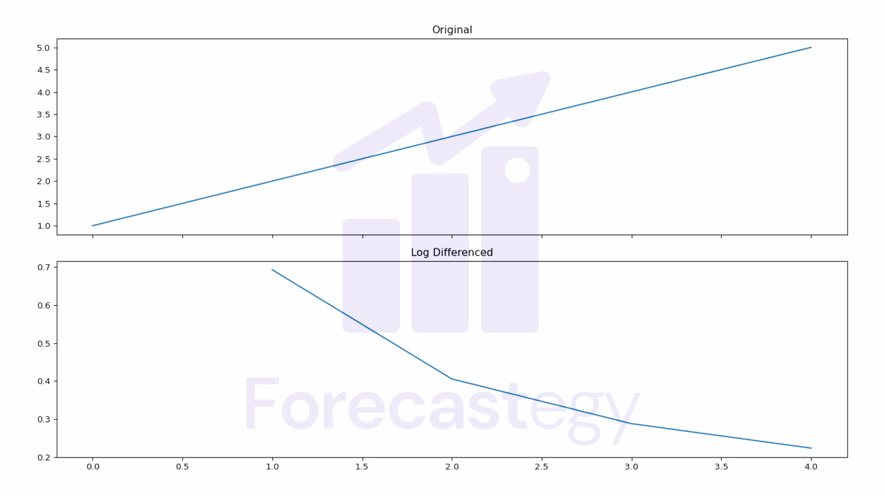
Log differencing involves taking the logarithm of a time series and then taking the first-order difference of the resulting sequence.
It’s a very common transformation in finance, where the log difference of a time series is often used to model the returns of a stock or other financial instrument.
Pandas
In Pandas, we can perform log differencing by calling the np.log() method and then taking the first-order difference.
import pandas as pd
import numpy as np

ts = pd.Series([1, 2, 3, 4, 5])

ts_diff = np.log(ts).diff()

print(ts_diff)
| log_diff | |
|---|---|
| 0 | nan |
| 1 | 0.693147 |
| 2 | 0.405465 |
| 3 | 0.287682 |
| 4 | 0.223144 |
The np.log() function uses the natural logarithm, which is the logarithm to the base e.
In case you have zeros in your time series, you can use the np.log1p() function instead.
This will add 1 to each value before taking the log, which will prevent it from returning infinite values.
import pandas as pd

ts = pd.Series([1, 2, 3, 4, 5])

ts_diff = np.log1p(ts).diff()

print(ts_diff)
| log1p_diff | |
|---|---|
| 0 | nan |
| 1 | 0.405465 |
| 2 | 0.287682 |
| 3 | 0.223144 |
| 4 | 0.182322 |
Numpy
In Numpy, we can perform log differencing by calling the np.log() function and then calling the np.diff() function.
import numpy as np

ts = np.array([1, 2, 4, 8, 16])

ts_diff = np.diff(np.log(ts))

print(ts_diff)

# output
[0.69314718 0.40546511 0.28768207 0.22314355]
Polars
In Polars, we can perform log differencing by calling the log() method and then taking the first-order difference using the diff() method.
import polars as pl

ts = pl.Series([1, 2, 3, 4, 5])

ts_diff = ts.log().diff()

print(ts_diff)

# output
shape: (5,)
Series: '' [f64]
[
	null
	0.693147
	0.405465
	0.287682
	0.223144
]
To reproduce the log1p behavior, we can add 1 to the time series before taking the log.
import polars as pl

ts = pl.Series([1, 2, 3, 4, 5])

ts_diff = (ts+1).log().diff()

print(ts_diff)

# output
shape: (5,)
Series: '' [f64]
[
	null
	0.405465
	0.287682
	0.223144
	0.182322
]
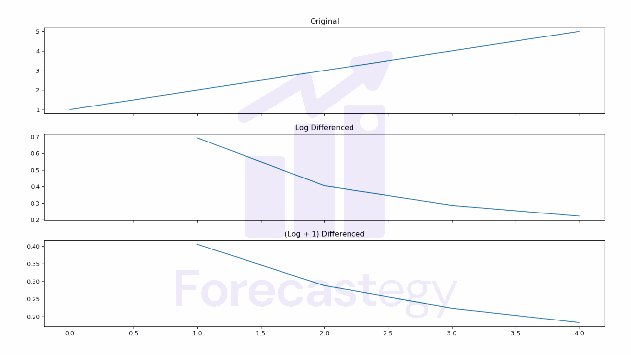
Again, look at the y-axis to see the difference between the original and the log differenced series.
Grouped Time Series Differencing
When you have a DataFrame with multiple time series in the long format, you can take their differences by grouping them first.
This can be useful in cases where you have multiple time series, such as the sales of different products in a store.
Pandas
In Pandas, we can perform grouped time series differencing by calling the groupby() method and then calling diff().
import pandas as pd

ts = pd.DataFrame({'values': [10, 20, 30, 40, 50, 100, 200, 300, 400, 500],
                   'groups': ['A', 'A', 'A', 'A', 'A', 'B', 'B', 'B', 'B', 'B']})

ts_diff = ts.groupby('groups').diff()
ts['diff'] = ts_diff['values']

print(ts)
| values | groups | diff |
|---|---|---|
| 10 | A | nan |
| 20 | A | 10 |
| 30 | A | 10 |
| 40 | A | 10 |
| 50 | A | 10 |
| 100 | B | nan |
| 200 | B | 100 |
| 300 | B | 100 |
| 400 | B | 100 |
| 500 | B | 100 |
Polars
In Polars, we can perform grouped time series differencing by calling the diff() method over the pl.col(ts) expression specifying the group column with the over() method.
import polars as pl

ts = pl.Series([10, 20, 30, 40, 50, 100, 200, 300, 400, 500])
groups = pl.Series(['A', 'A', 'A', 'A', 'A', 'B', 'B', 'B', 'B', 'B'])

ts = pl.DataFrame({'ts': ts, 'groups': groups})

ts_diff = ts.with_columns([pl.col('ts').diff().over(pl.col('groups')).alias('ts_diff')])

print(ts_diff)
| ts | groups | ts_diff |
|---|---|---|
| i64 | str | i64 |
| —– | ——– | ——— |
| 10 | A | null |
| 20 | A | 10 |
| 30 | A | 10 |
| 40 | A | 10 |
| 50 | A | 10 |
| 100 | B | null |
| 200 | B | 100 |
| 300 | B | 100 |
| 400 | B | 100 |
| 500 | B | 100 |
Fractional Differencing
Traditional n-order differencing makes the data stationary but, in the process, it tends to erase the dependence of the time series on its past values.
Fractional differencing was suggested by Marcos López de Prado, in the context of financial time series, as an alternative to differentiate them without erasing its memory structure.
We can apply it using the library fracdiff.
import numpy as np
from fracdiff import fdiff

ts = np.array([10, 20, 30, 40, 50, 100, 200, 300, 400, 500])

ts_diff = fdiff(ts, n=0.5)

#output
array([ 10.        ,  15.        ,  18.75      ,  21.875     ,
        24.609375  ,  67.0703125 , 139.32617188, 181.42089844,
       214.63470459, 243.0519104 ])
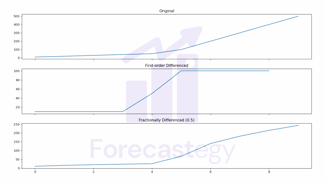
Tune the n parameter to find the coefficient that makes the data stationary while preserving as most as possible the memory structure of the time series.
You can do it by using statistical tests such as the Augmented Dickey-Fuller test or, if you plan to use the time series in a machine learning model, just tune this value as another hyperparameter in the validation set.