Time series data can be a valuable tool for predicting trends and making informed business decisions.
However, it can be difficult to analyze due to seasonal patterns and other fluctuations that can obscure underlying trends.
That’s where deseasonalizing comes in, allowing you to isolate trends and make more accurate predictions.
In this tutorial, we’ll explore two different approaches to deseasonalize time series data in Python: additive models and multiplicative models.
We’ll use the powerful Python library statsmodels to perform our analysis, and walk through the code step by step so that you can easily follow along.
What Is Seasonality?
If you already know what seasonality is, feel free to skip this section.
Seasonality in time series refers to a pattern that repeats itself at regular intervals over time.
This pattern could be daily, weekly, monthly, or even yearly, and it’s often caused by factors such as weather patterns, holidays, and other recurring events.
Let’s take the example of a company that sells ice cream.
The sales of ice cream may have a seasonal pattern, with higher sales during the summer and lower sales during the winter.
This is because people tend to eat more ice cream in the summer when it’s hot outside, and less in the winter when it’s cold.
This pattern of higher sales in the summer and lower sales in the winter is an example of seasonality in a time series.
Although the model doesn’t have information about the temperature, it can still capture the seasonal pattern in the data by looking at the time of year.
It just knows that in July (northern hemisphere) and January (southern hemisphere) it must adjust its predictions upwards, and in December (northern hemisphere) and June (southern hemisphere) it must adjust its predictions downwards.
In some cases, analyzing the data without this seasonal effect can help you better understand the underlying trends.
This is where deseasonalization comes in.
We can do this by using an additive model or a multiplicative model.
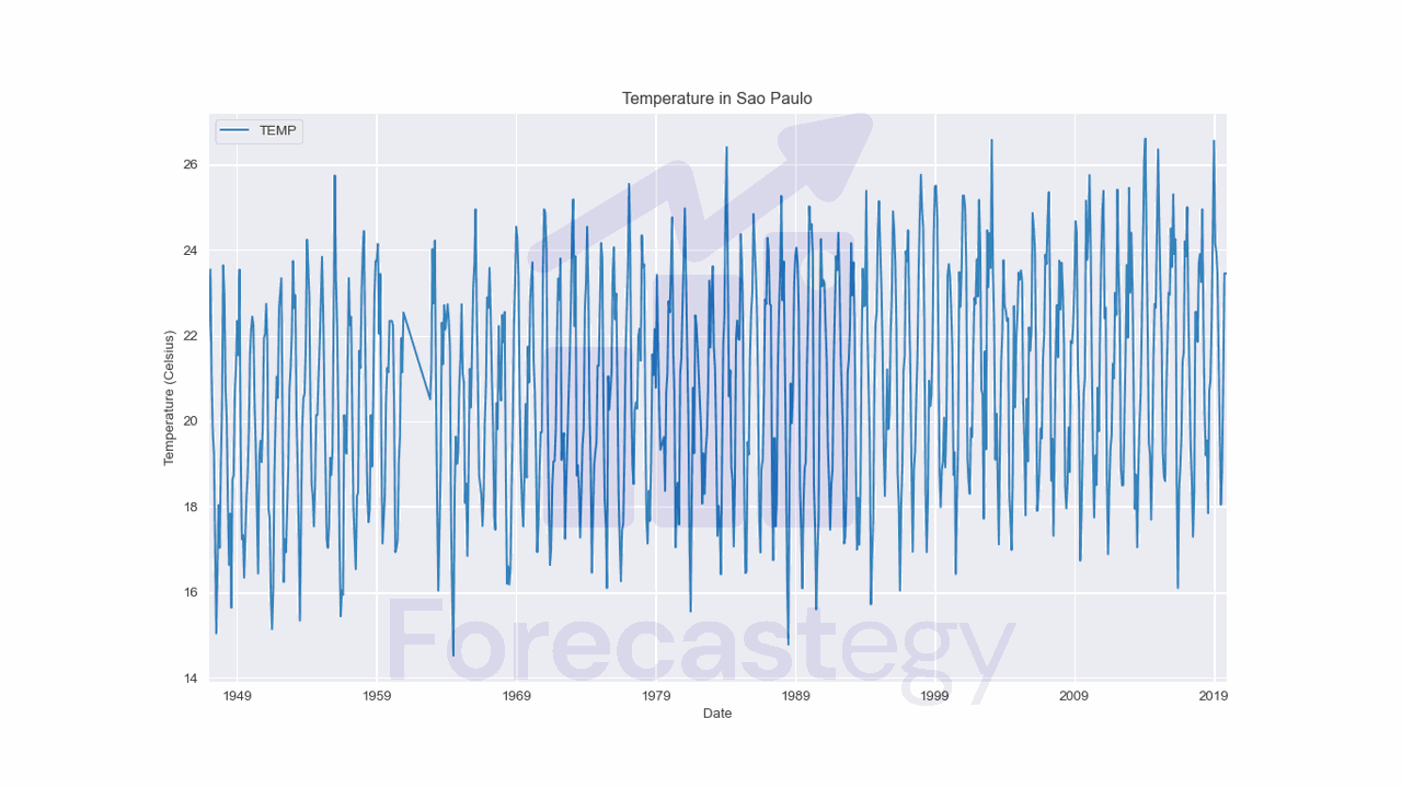
I will use a time series with monthly historical temperature in my city (Sao Paulo, Brazil) to demonstrate how you can perform deseasonalization in Python.
Here’s a preview of the data:
| TIMESTAMP | TEMP |
|---|---|
| 1980-12-01 00:00:00 | 22.63 |
| 1952-10-01 00:00:00 | 20.74 |
| 1991-01-01 00:00:00 | 23.3 |
| 2012-04-01 00:00:00 | 22.45 |
| 2018-02-01 00:00:00 | 23.25 |

Deseasonalizing With An Additive Model
In an additive model, the observations are modeled as a linear combination of the seasonal component, the trend component, and the error.
$$\mathrm{Y}(t) = \mathrm{T}\left(t\right) + \mathrm{S}\left(t\right) + \mathrm{e}\left(t\right)$$
where:
- $\mathrm{Y}(t)$ is the observation at time $t$
- $\mathrm{T}\left(t\right)$ is the trend at time $t$
- $\mathrm{S}\left(t\right)$ is the seasonal component at time $t$
- $\mathrm{e}\left(t\right)$ is the error at time $t$
The function seasonal_decompose from statsmodels decomposes a time series into these components.
from statsmodels.tsa.seasonal import seasonal_decompose

decomposition = seasonal_decompose(data['TEMP'], model='additive', period=12)
This function can’t handle missing values, so if you have it, you need to impute or remove them before using it.
You can do it easily with the interpolate method from pandas.
data['TEMP'].interpolate(inplace=True)
I like to sort my data by the timestamp before using it to be sure the function will do what I expect.
We want an additive model, so we set the model parameter to additive.
Our seasonality is monthly, so we set the period parameter to 12.
If your seasonality is:
- hourly, set
periodto 24 - weekdays, set
periodto 7 - daily, set
periodto 365 - weekly, set
periodto 52
You get the idea.
After the function runs, it returns a DecomposeResult object with attributes for trend and seasonal.
We just want the seasonal component, so we can access it with decomposition.seasonal.
To deseasonalize our data, we just need to subtract the seasonal component from the original data.
deseason_temp = data['TEMP'] - decomposition.seasonal
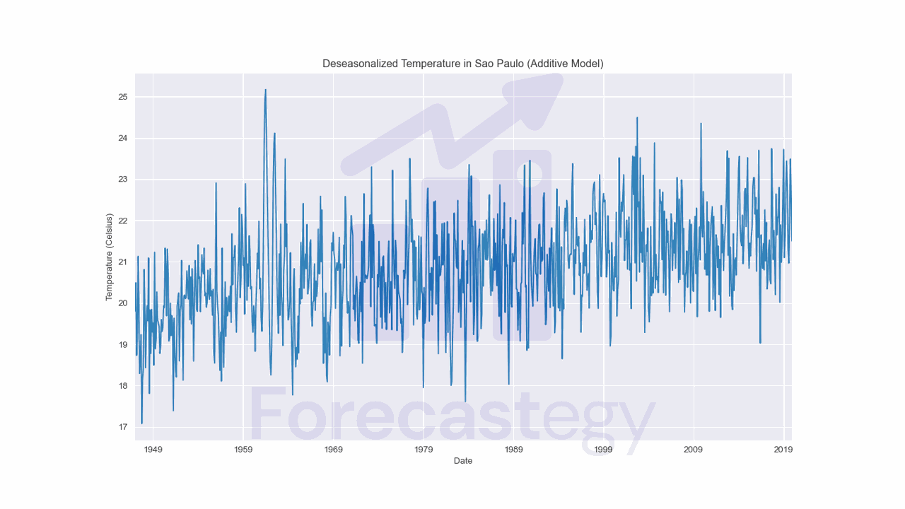
Notice that the plot seems more jagged than the original one. Now it doesn’t have a strong seasonal component, but we can see the trend more clearly.
Deseasonalizing With A Multiplicative Model
In a multiplicative model, the observations are modeled as a product of the seasonal component, the trend component, and the error.
$$\mathrm{Y}(t) = \mathrm{T}\left(t\right) \times \mathrm{S}\left(t\right) \times \mathrm{e}\left(t\right)$$
where:
- $\mathrm{Y}(t)$ is the observation at time $t$
- $\mathrm{T}\left(t\right)$ is the trend at time $t$
- $\mathrm{S}\left(t\right)$ is the seasonal component at time $t$
- $\mathrm{e}\left(t\right)$ is the error at time $t$
Deseasonalizing with a multiplicative model involves dividing the observed values by the seasonal component to obtain the deseasonalized values.
We can use the same seasonal_decompose function from statsmodels to obtain the seasonal component for a multiplicative model.
The only difference is that we need to set the model parameter to 'multiplicative'.
decomposition = seasonal_decompose(data['TEMP'], model='multiplicative', period=12)
To deseasonalize our data, we just need to divide the original data by the seasonal component.
deseason_temp = data['TEMP'] / decomposition.seasonal
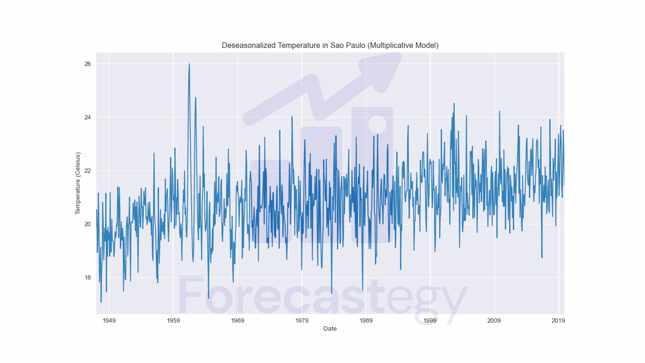
Again, we can see that the deseasonalized data has a clearer trend, without the influence of the seasonal component.
How To Choose Between An Additive Model And A Multiplicative Model?
In general, an additive model is more appropriate when the seasonal pattern in the data is consistent over time, regardless of whether the overall trend of the data is increasing or decreasing.
Let’s say we have a time series of monthly sales for a retail store.
The data shows that sales have a consistent increase each year during the holiday season (November and December).
This increase in sales is roughly the same regardless of the magnitude of the trend.
In this case, we can use an additive model to deseasonalize the data.
On the other hand, a multiplicative model is more appropriate when the seasonal fluctuations are proportional to the trend of the time series.
Let’s say we have a time series of monthly electricity usage for a household.
The data shows that usage increases during the summer months and decreases during the winter.
However, the increase in usage during the summer is larger when the overall electricity usage is higher (e.g. due to more people living in the household or using more appliances).
In this case, we can use a multiplicative model to deseasonalize the data since the amplitude of the seasonal component changes with the level of the trend.
Plot your data and use your domain knowledge (or ask domain experts) to decide which model is more appropriate.
And if you want to take the practical approach, you can try both models and see which one gives you better results according to your business objective.
If you are forecasting, for example, you can compare the forecasted values after deseasonalizing with both models and see which one gives you the best results.