Discovering outliers, unusual patterns or events in your time series data has never been easier!
In this tutorial, I’ll walk you through a step-by-step guide on how to detect anomalies in time series data using Python.
You won’t have to worry about missing sudden changes in your data or trying to keep up with patterns that change over time.
I’ll use website impressions data from Google Search Console as an example, but the techniques I cover will work for any time series data.
If you know a bit about Python programming and are familiar with libraries like pandas, numpy, and matplotlib, you’ll get a lot out of this tutorial.
Let’s get started!
What Is The Difference Between Anomalies And Outliers?
In the context of time series analysis, the terms “anomalies” and “outliers” are often used interchangeably. However, there is a subtle difference between the two terms.
Anomalies refer to data points that deviate from the expected pattern or trend in the time series.
These deviations can be due to various reasons, such as seasonality, external events, or underlying changes in the data-generating process.
Outliers, on the other hand, are data points that are statistically different from the majority of the data. They may or may not be part of the expected pattern or trend.
Outliers can be caused by measurement errors, extreme events, or other factors that lead to a significant deviation from the norm.
So, while there is a subtle difference between the terms, it’s important to note that both anomalies and outliers represent deviations from the norm in time series data.
In practice, the terms are often used interchangeably.
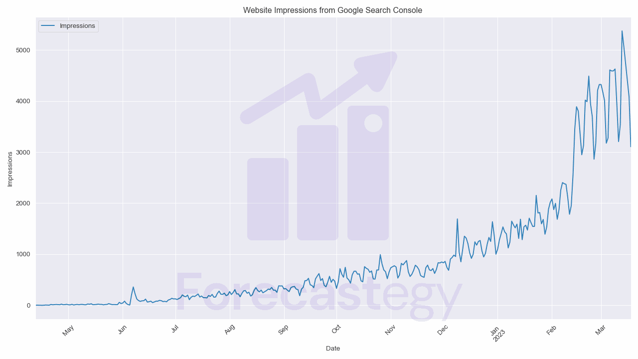
Loading The Impression Data
First, we need to load our dataset.
In this tutorial, we’ll be working with website impressions data from Google Search Console.
This data reflects the number of times specific pages on a website appeared in Google Search results.
By analyzing this data, a site owner can make informed decisions about optimizing the website for higher search engine rankings and increased organic traffic.
The dataset contains two columns: Date and Impressions.
We’ll use pandas to load the dataset and parse the Date column as a datetime object:
import pandas as pd
import numpy as np
import os

path = "your_data_path_here"
data = pd.read_csv(os.path.join(path, 'impressions.csv'), parse_dates=['Date'], usecols=['Date', 'Impressions'])
To prepare the data for statsforecast we need to have the Date and Impressions columns named ds and y respectively.
StatsForecast was created to be used with multiple time series, so it requires a unique identifier for each time series.
In our case we only have one time series, so we’ll just set the unique_id to 1 for all rows.
impressions = data.rename(columns={'Date': 'ds', 'Impressions': 'y'})
impressions['unique_id'] = 1
| ds | y | unique_id |
|---|---|---|
| 2022-04-12 00:00:00 | 0 | 1 |
| 2022-04-13 00:00:00 | 3 | 1 |
| 2022-04-14 00:00:00 | 2 | 1 |
| 2022-04-15 00:00:00 | 0 | 1 |
| 2022-04-16 00:00:00 | 0 | 1 |
Now, we’ll split our data into train and validation sets.
In this anomaly detection case, we don’t have labeled anomalies, so we can think about the validation set as simply the period of time where we want to detect anomalies.
Impressions on search tend to change on a weekly basis, so I’ll use the last 7 days of data as my validation set.
train = impressions.iloc[:-7]
valid = impressions.iloc[-7:]
In a deployment scenario, you can store the predictions for the next period and compare as you get new data.
Here, for example, I would make the predictions Sunday at 12:00 AM and run a job to compare the predictions with the actual data every day at 12:00 AM.
Training ARIMA For Anomaly Detection
We’ll use the AutoARIMA model from the StatsForecast library, which automatically selects the best ARIMA model for our data.
You can use any model that is able to make accurate predictions for your data with confidence intervals.
I chose ARIMA because it tends to work well with many types of time series data and outputs confidence intervals by default.
We’ll set the season_length parameter to 7, assuming a weekly seasonality in our data (traffic is much lower on weekends).
from statsforecast.models import AutoARIMA
from statsforecast import StatsForecast

model = StatsForecast(models=[AutoARIMA(season_length=7)],freq='D')
model.fit(train)
StatsForecast is a wrapper around the models, that take a list of models and train them on the data.
I am using only a single model, but you can use multiple models and compare the results.
After training the model, we use the forecast method to make predictions for the next 7 days or whatever period you want to detect anomalies.
For demonstration purposes, I’ll use a 99% confidence interval and merge the real values with the predictions.
The anomaly column will be 1 if the real value is outside the confidence interval and 0 otherwise.
p = model.forecast(7, level = [99])
p = p.merge(valid, on=['ds', 'unique_id'], how='left')
p['anomaly'] = ((p['y'] > p['AutoARIMA-hi-99']) | (p['y'] < p['AutoARIMA-lo-99'])).astype(int)
| ds | unique_id | AutoARIMA | AutoARIMA-lo-99 | AutoARIMA-hi-99 | y | anomaly |
|---|---|---|---|---|---|---|
| 2023-03-12 00:00:00 | 1 | 3470.78 | 3097.46 | 3844.11 | 3540 | 0 |
| 2023-03-13 00:00:00 | 1 | 4554.21 | 4107.09 | 5001.33 | 5373 | 1 |
| 2023-03-14 00:00:00 | 1 | 4684.89 | 4191.23 | 5178.55 | 5071 | 0 |
| 2023-03-15 00:00:00 | 1 | 4795.59 | 4275.59 | 5315.6 | 4739 | 0 |
| 2023-03-16 00:00:00 | 1 | 4681.26 | 4136.18 | 5226.34 | 4414 | 0 |

The confidence interval represents the range within which we expect the actual values to fall.
When a data point falls outside of this range, it suggests that there’s only a small chance that such an observation would occur due to normal variation in the data.
In other words, it’s highly likely that this data point is an anomaly.
This approach is effective because it’s statistically robust and considers the inherent uncertainty in time series forecasting.
By quantifying the uncertainty using confidence intervals, we can better identify which data points are truly unusual and not just a result of noise or random fluctuations in the data.
In production, this could raise an alert to the data scientist or engineer to investigate the anomaly.
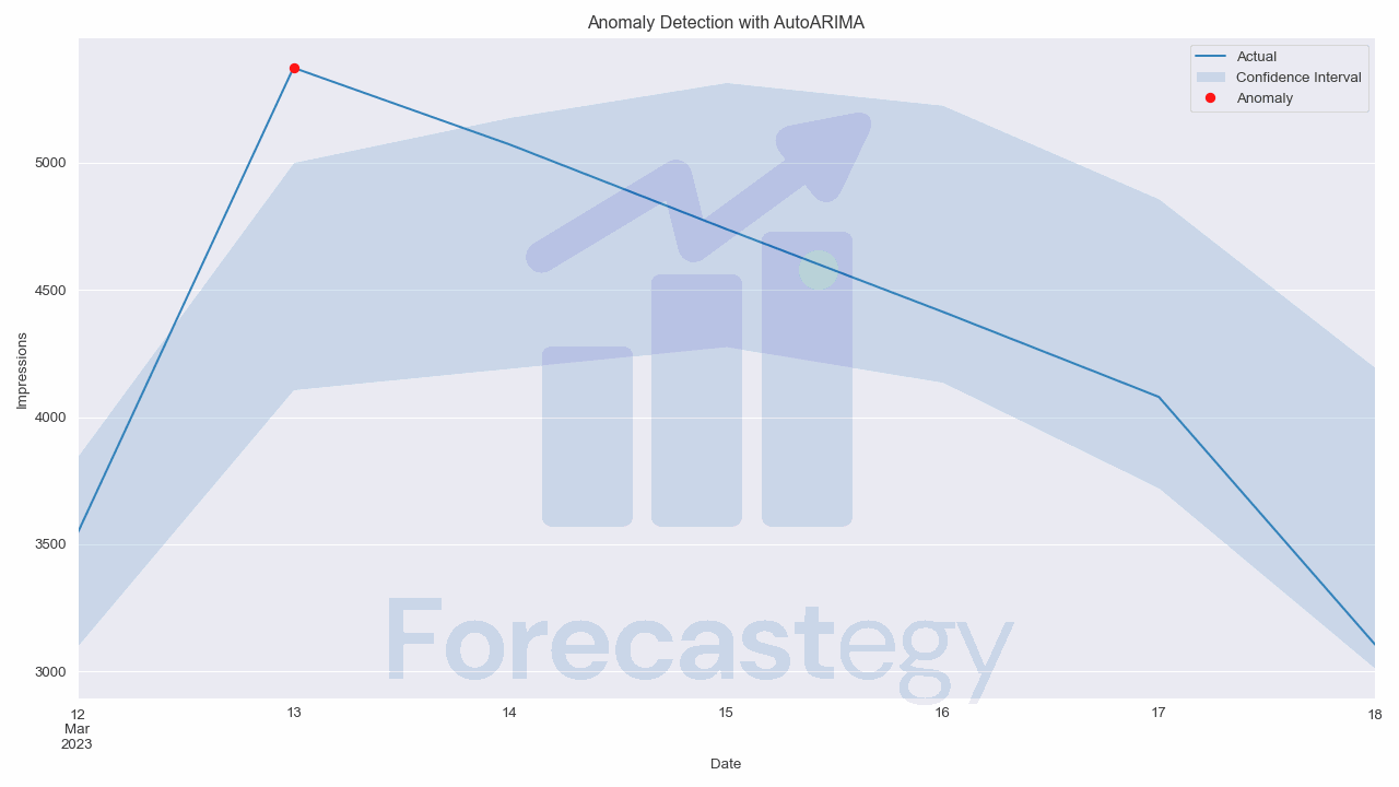
To generate a plot that highlights the anomalies, we can use the following code:
fig, ax = plt.subplots(1, 1, figsize=(1280/96, 720/96), dpi=96)
p.plot(x='ds', y='y', ax=ax)
ax.fill_between(p['ds'].values, p['AutoARIMA-hi-99'], p['AutoARIMA-lo-99'], alpha=0.2)

anomaly_indices = p[p['anomaly'] == 1].index
p.loc[anomaly_indices].plot(x='ds', y='y', ax=ax, style='ro')
plt.legend(['Actual', 'Confidence Interval', 'Anomaly'])
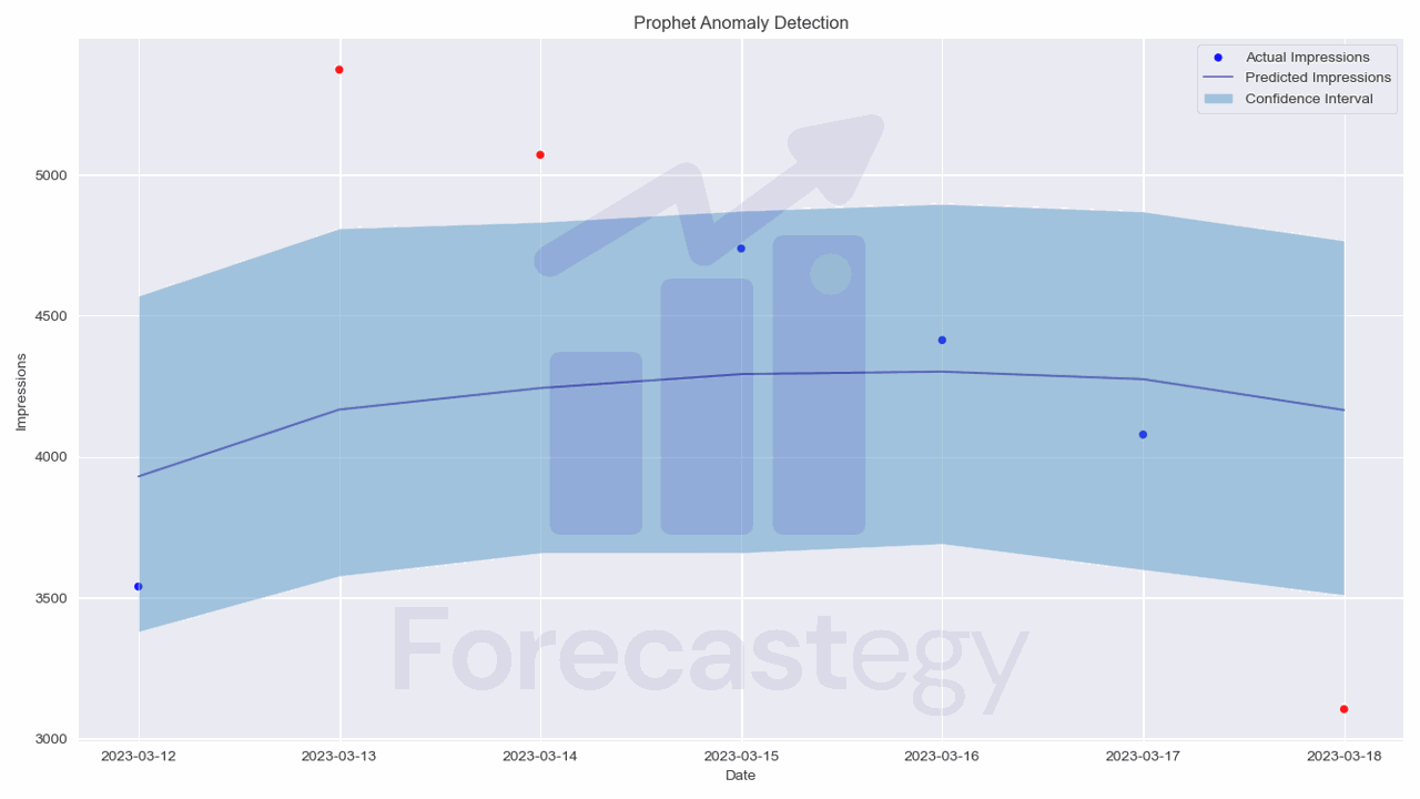
Training Facebook Prophet For Anomaly Detection
Now that we’ve seen how to implement anomaly detection using ARIMA, let’s explore another popular forecasting method: Facebook’s Prophet.
Prophet is a forecasting tool that is able to handle time series data with strong seasonal effects.
According to the creators, it’s also robust to missing data and shifts in the trend, making it a suitable choice for anomaly detection.
First, we need to install Prophet. We can do this using pip or conda:
pip install prophet
conda install -c conda-forge prophet
We’ll use the same dataset as before.
from fbprophet import Prophet

model = Prophet(interval_width=0.99,  daily_seasonality=True, weekly_seasonality=True)
Like before, we set the confidence interval to 99% and enable daily and weekly seasonality.
We then fit the model to our training data:
model.fit(train)
Prophet requires the input DataFrame to contain a ‘ds’ column for date and a ‘y’ column for the variable we wish to forecast, which is already the case here.
After training the model, we use the make_future_dataframe method to create a DataFrame that extends into the future for the period we want to detect anomalies (7 days in this case).
The include_history parameter is set to False to exclude the training data from the future DataFrame and make it easier to visualize the predictions.
We then use the predict method to make predictions for the specified future period:
future = model.make_future_dataframe(periods=7, include_history=False)
forecast = model.predict(future)
forecast = forecast.merge(impressions, on='ds', how='left')
| ds | trend | yhat_lower | yhat_upper | trend_lower | trend_upper | additive_terms | additive_terms_lower | additive_terms_upper | daily | daily_lower | daily_upper | weekly | weekly_lower | weekly_upper | multiplicative_terms | multiplicative_terms_lower | multiplicative_terms_upper | yhat | y | unique_id |
|---|---|---|---|---|---|---|---|---|---|---|---|---|---|---|---|---|---|---|---|---|
| 2023-03-12 00:00:00 | 4121.52 | 3341.99 | 4603.31 | 4120.54 | 4122.84 | -191.169 | -191.169 | -191.169 | -53.0502 | -53.0502 | -53.0502 | -138.119 | -138.119 | -138.119 | 0 | 0 | 0 | 3930.35 | 3540 | 1 |
| 2023-03-13 00:00:00 | 4164.38 | 3565.06 | 4798.81 | 4160.26 | 4168.35 | 3.39548 | 3.39548 | 3.39548 | -53.0502 | -53.0502 | -53.0502 | 56.4457 | 56.4457 | 56.4457 | 0 | 0 | 0 | 4167.78 | 5373 | 1 |
| 2023-03-14 00:00:00 | 4207.24 | 3641.35 | 4895.7 | 4200.36 | 4214.96 | 36.6028 | 36.6028 | 36.6028 | -53.0502 | -53.0502 | -53.0502 | 89.653 | 89.653 | 89.653 | 0 | 0 | 0 | 4243.84 | 5071 | 1 |
| 2023-03-15 00:00:00 | 4250.1 | 3719.98 | 4847.31 | 4239.7 | 4262.59 | 43.395 | 43.395 | 43.395 | -53.0502 | -53.0502 | -53.0502 | 96.4452 | 96.4452 | 96.4452 | 0 | 0 | 0 | 4293.49 | 4739 | 1 |
| 2023-03-16 00:00:00 | 4292.95 | 3707.74 | 4895.56 | 4278.39 | 4310.35 | 9.22503 | 9.22503 | 9.22503 | -53.0502 | -53.0502 | -53.0502 | 62.2753 | 62.2753 | 62.2753 | 0 | 0 | 0 | 4302.18 | 4414 | 1 |
The forecast DataFrame includes a column ‘yhat’ with the forecast, as well as columns for components and uncertainty intervals ‘yhat_lower’ and ‘yhat_upper’.
I merged the original data to make it easier to highlight the anomalies.
We will consider a data point to be an anomaly if it falls outside the 99% confidence interval:
forecast['anomaly'] = ((valid['y'] > forecast['yhat_upper']) | (valid['y'] < forecast['yhat_lower'])).astype(int)
How To Choose The Right Confidence Interval?
When we don’t have labeled anomalies, we need to trust our instincts, knowledge about the topic, and the needs of our business.
Start by trying different confidence intervals to find the best balance between finding real anomalies and not getting too many false alarms.
A smaller confidence interval, like 90%, will be more sensitive, finding more anomalies but maybe giving you more false alarms too.
A larger confidence interval, like 99%, will be less sensitive, finding fewer anomalies but giving fewer false alarms.
By testing a range of confidence intervals, you can figure out which one works best for your situation.
Looking at past data can help you understand the normal ups and downs and how often real anomalies happen.
For example, if you see that most real anomalies in the past were outside a 95% confidence interval, you might want to use a similar confidence interval now.
Data can change, so it’s important to check your confidence interval from time to time to make sure it still works well for your situation.
Think about the costs of missing a real anomaly (false negative) or mistakenly saying a normal data point is an anomaly (false positive).
Just be careful not to get too many alerts, as you might start ignoring them.
How To Evaluate The Performance Of Anomaly Detection Models?
Figuring out how well an anomaly detection model works depends on if you have labeled anomalies or not.
When you do have labeled anomalies, you can use common supervised learning measurements like precision, recall, and F1 score.
Precision shows the percentage of true positive anomalies found among all the data points that the model said were anomalies.
On the other hand, recall measures the model’s ability to find all the true anomalies in the dataset.
The F1 score is a balance between precision and recall, as it’s the harmonic mean of the two metrics.
Take into account the cost of missing a true anomaly (false negative) or incorrectly flagging a normal data point as an anomaly (false positive).
When you don’t have labeled anomalies, figuring out if your model works well can be tough.
One way to check is by looking at the detected anomalies and confidence intervals together with the original time series data.
By doing this, you can see if the anomalies your model found make sense based on what you know about the data.
It’s also important to think about how stable your model is.
You want to make sure that your model still works well when there are small changes in the data.
Talking to experts who know a lot about the data can help you understand if the anomalies your model found are what they expect to see.
They can give you feedback on whether your model’s results match their understanding of the data and the normal patterns that should be happening.