
Are you looking to train a Random Forest using XGBoost for classification or regression tasks but aren’t sure where to start?
In this tutorial, I will first briefly explain the mechanisms behind XGBoost and Random Forest and highlight their differences.
Then, I’ll guide you through a step-by-step process of training an XGBoost Random Forest for both classification and regression tasks using a real-world dataset.
By the end of this tutorial, you’ll be well-equipped to tackle your own projects with confidence and expertise.
So, let’s dive in and start exploring!
Standard XGBoost vs Random Forest
Before we dive into the code, let’s first understand the mechanisms behind XGBoost and Random Forest.
XGBoost is an implementation of gradient boosting that uses decision trees as base learners.
Boosting, in a nutshell, is a sequential process where each subsequent model attempts to correct the errors of the previous model.
The models are built sequentially, with each new model being trained to correct the errors made by the combination of the previous ones.
This sequential nature requires careful tuning and a lot of computational resources.
On the other hand, Random Forest is a bagging technique mixed with the random subspace method, also applied to decision trees.
Bagging, or bootstrap aggregating, involves training many models on different subsets of the original data (sampled with replacement) and then aggregating their predictions.
The Random Forest goes one step further and randomly selects a subset of features at each split point of the decision tree.
The models are built independently, which allows for parallel computation.
Random Forest is particularly effective when dealing with high variance in data, as the aggregation process tends to smooth out the noise.
In summary, the main difference between XGBoost and Random Forest lies in how they build and combine the models: XGBoost builds one tree at a time, where each new tree helps to correct errors made by the combination of previously trained trees.
On the other hand, Random Forest builds many trees over randomly sampled subsets of the data and features, and then averages their predictions.
Training XGBoost Random Forest For Classification
Let’s now dive into training a Random Forest using XGBoost for a classification task.
We will use the XGBRFClassifier class from the xgboost library.
This is an interface that imitates the sklearn API, so it should be familiar to you if you’ve used scikit-learn before.
First, we need to import the necessary libraries and load our data.
We’ll use the Red Wine dataset, which we can load using the pandas library.
This dataset contains chemical features measured from red wines (alcohol, pH, citric acid, etc.) and a quality score between 3 and 8. Higher is better.
Our goal is to train a model that can predict the quality score of a wine given its chemical features.
This task can be treated as a classification or a regression, so we’ll train both types of models.
import pandas as pd
from sklearn.model_selection import train_test_split
from xgboost import XGBRFClassifier

# Load the dataset
url = "https://archive.ics.uci.edu/ml/machine-learning-databases/wine-quality/winequality-red.csv"
data = pd.read_csv(url, sep=";")
Next, we split our data into features (X) and target (y).
X = data.drop('quality', axis=1)
y = data['quality'] - data['quality'].min()

# Split the data into train and test sets
X_train, X_test, y_train, y_test = train_test_split(X, y, test_size=0.2, random_state=42)
Notice that I subtracted the minimum quality score from the target variable.
XGBoost expects the classes to be numbered from 0 to n_classes - 1, so we need to make sure that our target variable is in this format.
Now, we can train our XGBoost Random Forest Classifier.
We’ll instantiate the XGBRFClassifier class and fit it to our training data.
# Instantiate the XGBRFClassifier
xgbrf_classifier = XGBRFClassifier(n_estimators=100, max_depth=100)

# Fit the classifier to the training data
xgbrf_classifier.fit(X_train, y_train)
You can make predictions with this model by calling the predict method on xgbrf_classifier with new data.
from sklearn.metrics import classification_report

p = xgbrf_classifier.predict(X_test)
classification_report(y_test, p)
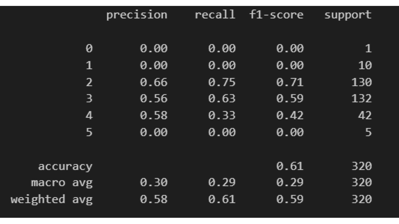
In the code above, we used the classification_report function from sklearn to evaluate the performance of our model.
This function shows us the precision, recall, and F1 score for each class in our dataset.
If you want the probabilities of each class instead of only the most likely class, you can use the predict_proba method instead.
p = xgbrf_classifier.predict_proba(X_test)
Training XGBoost Random Forest For Regression
Now, let’s see how we can train an XGBoost Random Forest for a regression task.
The process is very similar to the classification task, but this time we’ll use the XGBRFRegressor class from the xgboost library.
To save time, I’ll use the same dataset as before, but now we don’t need to subtract the minimum quality score from the target variable.
X = data.drop('alcohol', axis=1)
y = data['alcohol']

# Split the data into train and test sets
X_train, X_test, y_train, y_test = train_test_split(X, y, test_size=0.2, random_state=42)
Now, we can train our XGBoost Random Forest Regressor.
We’ll instantiate the XGBRFRegressor class and fit it to our training data.
# Instantiate the XGBRFRegressor
xgbrf_regressor = XGBRFRegressor(n_estimators=100, max_depth=100)

# Fit the regressor to the training data
xgbrf_regressor.fit(X_train, y_train)
Like before, you can make predictions with this model by calling the predict method on xgbrf_regressor with new data.
from sklearn.metrics import mean_squared_error

p = xgbrf_regressor.predict(X_test)
mean_squared_error(y_test, p, squared=False)
The mean_squared_error function from sklearn with squared=False returns the root mean squared error (RMSE) of our model.
Top Hyperparameters To Tune
I sometimes say that Random Forests are perfect models for “lazy days”.
They are easy to train and basically require a single hyperparameter: the number of trees.
In the XGBoost Random Forest implementation, n_estimators refers to the number of trees you want to build.
Higher values of n_estimators create more trees, which can lead to better performance.
However, adding more trees can slow down the training process.
Furthermore, after a certain point, adding more trees will not improve the performance.
In the plot below, we can see that the performance of the model increases as we add more trees, but it starts to plateau after 1000.
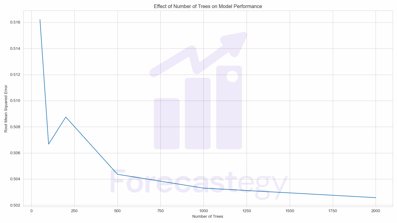
Still, this is why I say it’s a perfect model for lazy days: you can just set n_estimators to a high value and let the model do its thing.
A secondary hyperparameter you can tune is max_depth.
max_depth is the maximum depth of each tree and can be seen as a regularization hyperparameter.
The deeper the tree, the more splits it has and it captures more information about the data.
For gradient boosting, shallow trees are preferred, but for Random Forests, deeper trees are better.
This is why I set it to 100 in the code above, as the default value is 6 (because it’s the default value for gradient boosting).
I usually prefer to regularize my Random Forests by increasing the number of trees instead of limiting their depth.
You usually don’t want to set a limit on the depth of the trees, but if you need to limit the number of trees, limiting their depth might help avoid overfitting.
The “ideal” Random Forest has infinite trees with infinite depth.
In practice, we obviously can’t afford to train or infer infinite trees, so we have to make some trade-offs.