
You’ve chosen XGBoost as your algorithm, and now you’re wondering: “How do I figure out which features are the most important in my model?”
That’s what ‘feature importance’ is all about. It’s a way of finding out which features in your data are doing the heavy lifting when it comes to your model’s predictions.
Understanding which features are important can help you interpret your model better.
Maybe you’ll find a feature you didn’t expect to be important. Or maybe you’ll see that a feature you thought was important isn’t really doing much at all.
In this tutorial, we’ll dive into how to implement this in your code and interpret the results.
How Is Feature Importance Calculated in XGBoost?
Now that you understand what feature importance is, let’s talk about the different types of feature importance you can get with XGBoost.
There are five main types: ‘weight’, ‘gain’, ‘cover’, ’total_gain’, and ’total_cover’.
Let’s break each one down:
-
Weight: This is the simplest type of feature importance. It’s just the number of times a feature is used to split the data across all trees. If a feature is used a lot, it has a high weight.
-
Gain: This is a bit more complex. Gain measures the average improvement in (training set) loss brought by a feature. In other words, it tells you how much a feature helps to make accurate predictions in your training data.
-
Cover: Cover measures the number of data points a given feature affects. This is done via taking the average of the hessian values of all splits the feature is used in.
-
Total_gain: This is similar to gain, but instead of the average, it gives you the total improvement brought by a feature.
-
Total_cover: This is like cover, but it gives you the total number, rather than the average.
So, when should you use each type?
Unfortunately, there’s no one-size-fits-all answer.
I like to compute all of them and then use my best judgement to decide which one is most useful for my particular problem.
Implementing XGBoost Feature Importance in Python
We’ll be using the Red Wine dataset from UCI for this example.
This dataset contains information about various attributes of red wines, such as ‘fixed acidity’, ‘volatile acidity’, ‘citric acid’, etc.
The task is to predict the quality of the wine based on these attributes.
First, you’ll need to import the necessary libraries.
We’ll need pandas for data manipulation, XGBoost for our model, and matplotlib for plotting our feature importances later.
import pandas as pd
from xgboost import XGBRegressor
import matplotlib.pyplot as plt
Next, let’s load our dataset. We’ll use pandas’ read_csv function for this.
df = pd.read_csv('winequality-red.csv', delimiter=';')
| fixed acidity | volatile acidity | citric acid | residual sugar | chlorides | free sulfur dioxide | total sulfur dioxide | density | pH | sulphates | alcohol | quality |
|---|---|---|---|---|---|---|---|---|---|---|---|
| 7.4 | 0.7 | 0 | 1.9 | 0.076 | 11 | 34 | 0.9978 | 3.51 | 0.56 | 9.4 | 5 |
| 7.8 | 0.88 | 0 | 2.6 | 0.098 | 25 | 67 | 0.9968 | 3.2 | 0.68 | 9.8 | 5 |
| 7.8 | 0.76 | 0.04 | 2.3 | 0.092 | 15 | 54 | 0.997 | 3.26 | 0.65 | 9.8 | 5 |
| 11.2 | 0.28 | 0.56 | 1.9 | 0.075 | 17 | 60 | 0.998 | 3.16 | 0.58 | 9.8 | 6 |
| 7.4 | 0.7 | 0 | 1.9 | 0.076 | 11 | 34 | 0.9978 | 3.51 | 0.56 | 9.4 | 5 |
Now, we need to separate our features (X) from our target variable (y).
In this case, we’re trying to predict the ‘quality’ column.
So, we’ll drop that column from our dataframe and assign it to y.
Then, we’ll assign the rest of the dataframe to X.
X = df.drop('quality', axis=1)
y = df['quality']
Here I am not splitting the data into training and test sets to keep things brief, so assume that we have already done that.
The native feature importances are calculated using the training set only, as it’s the data used to create the decision trees.
Next, we’ll create our XGBoost model. We’ll use the XGBRegressor for this example.
Everything is valid for XGBClassifier as well.
Let’s use the default hyperparameters.
model = XGBRegressor()
Then, we fit our model to the data.
model.fit(X, y)
Now comes the fun part: getting our feature importances.
XGBoost sklearn API makes this easy with the feature_importances_ attribute.
To make it easier to understand, let’s put everything into a pandas Series where the index is the feature name and the values are the feature importances.
importances = model.feature_importances_
pd.Series(importances, index=X.columns).sort_values()
| 0 | |
|---|---|
| fixed acidity | 0.0356799 |
| density | 0.051082 |
| free sulfur dioxide | 0.0526365 |
| chlorides | 0.0537856 |
| residual sugar | 0.055074 |
| citric acid | 0.0559636 |
| pH | 0.0683643 |
| total sulfur dioxide | 0.0783635 |
| sulphates | 0.0954391 |
| volatile acidity | 0.0955693 |
| alcohol | 0.358042 |
As you can see, the ‘alcohol’ feature is by far the most important, with the highest feature importance score of 0.358042.
By default, XGBoost will use the ‘gain’ type of feature importance.
Let’s try other types to see if we get different results.
You need to change it in the model initialization using the importance_type parameter.
model = XGBRegressor(importance_type='weight')
model.fit(X, y)

importances = model.feature_importances_
pd.Series(importances, index=X.columns).sort_values()
| 0 | |
|---|---|
| free sulfur dioxide | 0.0671536 |
| alcohol | 0.0680961 |
| pH | 0.0713949 |
| citric acid | 0.0798775 |
| residual sugar | 0.0803487 |
| sulphates | 0.0838831 |
| density | 0.0933082 |
| total sulfur dioxide | 0.0937795 |
| chlorides | 0.0951932 |
| volatile acidity | 0.111216 |
| fixed acidity | 0.155749 |
This time, the ‘fixed acidity’ feature is the most important, with a feature importance score of 0.155749.
This means it’s the one that’s used the most to split the data across all trees.
Be careful, as this can be misleading.
In the case of high cardinality categorical features, the ‘weight’ type of feature importance will be biased towards those features, as they naturally have more splits.
Random Forests suffer from the same problem.
Here is the same example with the ‘cover’ type of feature importance for completion.
model = XGBRegressor(importance_type='cover')
| 0 | |
|---|---|
| fixed acidity | 0.0465268 |
| free sulfur dioxide | 0.0672191 |
| citric acid | 0.0774046 |
| volatile acidity | 0.0809456 |
| residual sugar | 0.0822461 |
| sulphates | 0.0887277 |
| total sulfur dioxide | 0.0980716 |
| chlorides | 0.0999913 |
| pH | 0.104945 |
| density | 0.125591 |
| alcohol | 0.128332 |
Finally, here are the results for all types (averaged, not doing the total ones to keep it brief):
| weight | gain | cover | |
|---|---|---|---|
| fixed acidity | 0.155749 | 0.0356799 | 0.0465268 |
| volatile acidity | 0.111216 | 0.0955693 | 0.0809456 |
| citric acid | 0.0798775 | 0.0559636 | 0.0774046 |
| residual sugar | 0.0803487 | 0.055074 | 0.0822461 |
| chlorides | 0.0951932 | 0.0537856 | 0.0999913 |
| free sulfur dioxide | 0.0671536 | 0.0526365 | 0.0672191 |
| total sulfur dioxide | 0.0937795 | 0.0783635 | 0.0980716 |
| density | 0.0933082 | 0.051082 | 0.125591 |
| pH | 0.0713949 | 0.0683643 | 0.104945 |
| sulphates | 0.0838831 | 0.0954391 | 0.0887277 |
| alcohol | 0.0680961 | 0.358042 | 0.128332 |
Visualizing XGBoost Feature Importance
Finally, let’s plot our feature importances to make them easier to understand.
We’ll create a bar plot with our features on the x-axis and their importance on the y-axis.
As we have our feature importances organized in a pandas Dataframe, we can easily plot them using the integrated matplotlib functions.
res.plot.barh(figsize=(1280/96, 720/96), title='Feature importance')
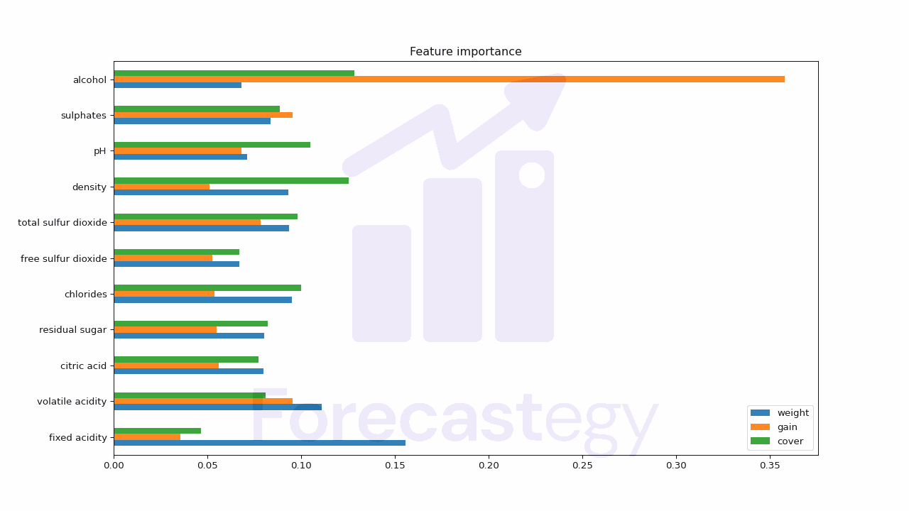
Here I plotted all the types of feature importance for comparison, but you can plot only one if you want.
The biggest downside of these feature importances is that they don’t tell the direction of the relationship, only the strength of it.
So we don’t know if a feature is positively or negatively correlated with the target variable.
In any case, it’s still useful to get a general idea of which features are important.