Interpreting and identifying crucial features in machine learning models can be a tough nut to crack, especially when dealing with black-box models.
In this tutorial, we will dive deep into understanding global and local feature importance in Random Forests.
We will explore several techniques and tools to analyze and interpret these importances, making our models more transparent and reliable.
Let’s use the Red Wine Quality dataset from the UCI Machine Learning Repository to learn the techniques.
import pandas as pd
from sklearn.model_selection import train_test_split

url = "https://archive.ics.uci.edu/ml/machine-learning-databases/wine-quality/winequality-red.csv"
wine_data = pd.read_csv(url, sep=";")
wine_data['quality'] = wine_data['quality']

X = wine_data.drop('quality', axis=1)
y = wine_data['quality']

X_train, X_test, y_train, y_test = train_test_split(X, y, test_size=0.3, random_state=42)
| fixed acidity | volatile acidity | citric acid | residual sugar | chlorides | free sulfur dioxide | total sulfur dioxide | density | pH | sulphates | alcohol |
|---|---|---|---|---|---|---|---|---|---|---|
| 8.6 | 0.22 | 0.36 | 1.9 | 0.064 | 53 | 77 | 0.99604 | 3.47 | 0.87 | 11 |
| 12.5 | 0.46 | 0.63 | 2 | 0.071 | 6 | 15 | 0.9988 | 2.99 | 0.87 | 10.2 |
| 7.2 | 0.54 | 0.27 | 2.6 | 0.084 | 12 | 78 | 0.9964 | 3.39 | 0.71 | 11 |
| 6.4 | 0.67 | 0.08 | 2.1 | 0.045 | 19 | 48 | 0.9949 | 3.49 | 0.49 | 11.4 |
| 7.5 | 0.58 | 0.14 | 2.2 | 0.077 | 27 | 60 | 0.9963 | 3.28 | 0.59 | 9.8 |
High Cardinality Bias In Random Forests
Before we dive into the code, it’s important to understand the high cardinality bias.
This bias is a common problem in Random Forest models, where the model tends to overestimate the importance of features with a high number of unique values.
It happens because the algorithm uses the gain in impurity reduction as a proxy for feature importance.
However, when a feature has a high number of unique values, the gain in impurity reduction is artificially inflated due to the fact that the model is able to split on the feature more often.
It’s important to keep this in mind when interpreting feature importance plots, as it can lead to incorrect conclusions about the importance of features in the context of the model.
If you see a feature with high importance that doesn’t seem to be relevant to the problem, check if it has a high number of unique values.
Global Vs Local Feature Importance Methods
Global feature importance refers to the overall importance of a feature across all instances in the dataset, while local feature importance refers to the importance of a feature for a specific instance.
We will work with both types of feature importance in this tutorial.
Built-in Feature Importance With Scikit-Learn
Scikit-learn provides a built-in feature importance method for Random Forest models.
According to the documentation, this method is based on the decrease in node impurity.
In plain English, imagine you’re playing a guessing game with your friends, and you have a set of questions to ask to figure out the answer.
In a Random Forest, the questions are like the features in the model.
Some questions help you eliminate more possibilities than others.
The assumption is that features that help you eliminate more possibilities quickly are more important because they help you get closer to the correct answer faster
It’s very simple to get these feature importances with Scikit-learn:
from sklearn.ensemble import RandomForestRegressor

rf = RandomForestRegressor(n_estimators=100, random_state=42)
rf.fit(X_train, y_train)

global_importances = pd.Series(rf.feature_importances_, index=X_train.columns)
global_importances.sort_values(ascending=True, inplace=True)
global_importances.plot.barh(color='green')
plt.xlabel("Importance")
plt.ylabel("Feature")
plt.title("Global Feature Importance - Built-in Method")
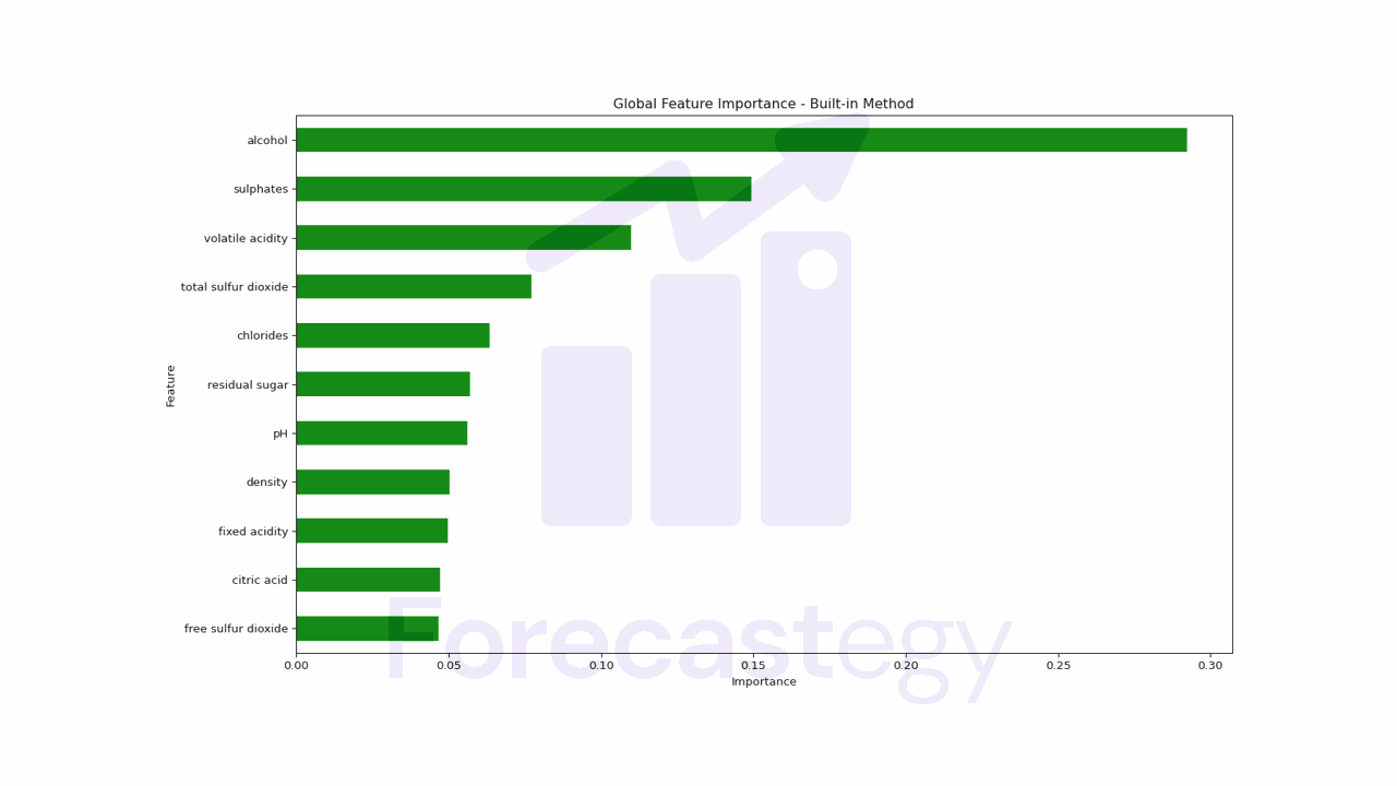
We just access the feature_importances_ attribute of the model and plot the results.
Alcohol and sulphates are the most important features in the model according to this method.
Keep this in mind so we can compare the results of the other methods.
There is no single best method, all of them are just estimates based on different assumptions.
A downside of this method is that it doesn’t provide any information about the direction of the relationship between the feature and the target.
In other words, it doesn’t tell us if more alcohol or sulphates are associated with higher quality wine or vice versa.
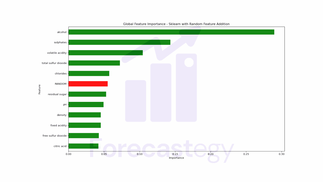
Built-in Scikit-learn Method With A Random Feature
A simple way to make this method more robust is to add a random feature to the dataset and see if it gets a high importance score.
The random feature acts as a benchmark against which the importance of the actual features can be compared.
If a real feature has lower importance than the random feature, it could indicate that its importance is just due to chance.
To use this method we just need to add a random column to the dataset and retrain the model.
import numpy as np

X_train_random = X_train.copy()
X_train_random["RANDOM"] = np.random.RandomState(42).randn(X_train.shape[0])

rf_random = RandomForestRegressor(n_estimators=100, random_state=42)
rf_random.fit(X_train_random, y_train)

global_importances_random = pd.Series(rf_random.feature_importances_, index=X_train_random.columns)
global_importances_random.sort_values(ascending=True, inplace=True)

In this case, any feature below the random feature, like residual sugar, should be put into question.
Permutation Feature Importance
Permutation feature importance is another technique to estimate the importance of each feature in a Random Forest model by measuring the change in the model’s performance when the feature’s values are randomly shuffled.
The permutation is done after the model is trained, using an out-of-sample dataset.
It works by following these steps:
- Train a machine learning model using the original dataset.
- Evaluate the model’s performance on a validation set and store the performance metric as baseline.
- For each feature:
- Create a copy of the validation set, and shuffle the values of the selected feature.
- Evaluate the model’s performance on the shuffled dataset and calculate the change in performance compared to the baseline.
- Average the change in performance over multiple iterations to obtain a stable estimate of the feature’s importance.
- Rank the features based on their importance scores.
One of the advantages of this method is that it can be used with any model, not just Random Forests, which makes the results between models more comparable.
Scikit-learn provides a built-in function to calculate it.
from sklearn.inspection import permutation_importance

rf = RandomForestRegressor(n_estimators=100, random_state=42)
rf.fit(X_train, y_train)

result = permutation_importance(rf, X_test, y_test, n_repeats=10, random_state=42)

perm_importances = result.importances_mean
perm_std = result.importances_std
sorted_idx = perm_importances.argsort()
feature_names = X_test.columns

pd.DataFrame({'Importance': perm_importances, 'Std': perm_std}, index=feature_names[sorted_idx]).sort_values('Importance',ascending=True)
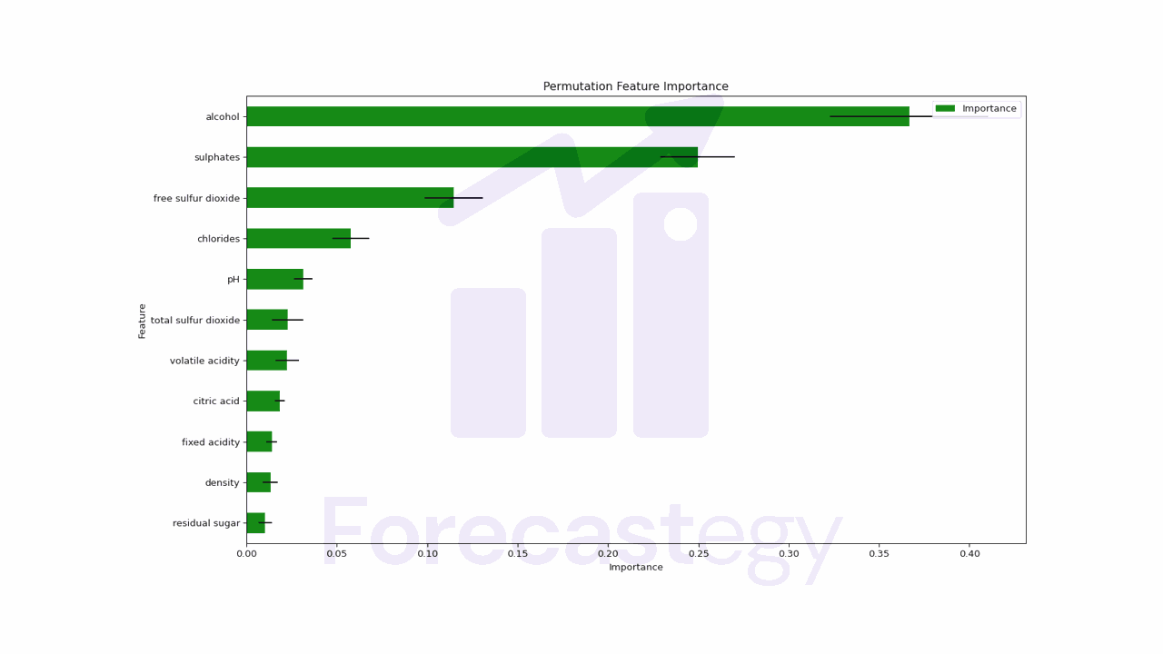
We have the average importance of each feature and the standard deviation of the importance scores.
To get more robust results, we can increase the n_repeats parameter, which is the number of times the permutation is repeated for each feature.
A drawback of this method is that it can be very slow to compute, especially for datasets with hundreds of features.
We still don’t have an indication of the direction of the relationship between the feature and the target with this method.
Random Forest Feature Importance With SHAP
SHAP is a method for interpreting the output of machine learning models based on game theory.
It provides a unified measure of feature importance that, like the permutation importance, can be applied to any model.
We get both global and local feature importance scores with SHAP.
The main drawback of it is that it can be computationally expensive, especially for large datasets or complex models.
It’s my favorite method because it provides a lot of information about the model.
To use it you need to install the shap package with pip or conda.
pip install shap
conda install -c conda-forge shap
Then you can simply pass the model to the shap.Explainer function and use the shap_values to plot the results.
Usually the explanations are calculated using the training set.
import shap

explainer = shap.Explainer(rf)
shap_values = explainer(X_train)

shap.plots.beeswarm(shap_values)
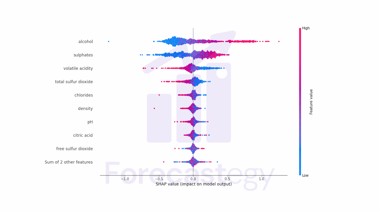
Besides showing the global feature importance, it also provides the direction of the relationship between the feature and the target.
Let’s take alcohol as an example.
Points that fall to the right of the middle line have a positive impact on the predictions, while points to the left have a negative impact.
Pink points are instances where the feature value is high, blue points are instances where the feature value is low.
Alcohol has many pink points on the right side, which means that it has a positive impact on the predictions.
More alcohol is associated with higher quality wine.
Volatile acidity is the opposite, it has many pink points on the left side, which means that higher values of this feature are associated with lower quality wine.
SHAP is great to get local explanations for individual predictions too, but at the moment it seems to be bugged for Random Forest models with scikit-learn.
Random Forest Path Feature Importance
Another way to understand how each feature contributes to the Random Forest predictions is to look at the decision tree paths that each instance takes.
It calculates the difference between the prediction value at the leaf node and the prediction values at the nodes that precede it to get the estimated contribution of each feature.
There is a really great explanation of this method by the author of the treeinterpreter package.
To use it in Python you need to install the treeinterpreter package with pip.
pip install treeinterpreter
Then you can use the treeinterpreter package to calculate the feature importances.
from treeinterpreter import treeinterpreter as ti

prediction, bias, contributions = ti.predict(rf, X_train)
The first argument is the trained model, the second is the dataset. I will use the training set here to keep consistency with the other methods.
You may get a lot of X has feature names, but DecisionTreeRegressor was fitted without feature names warnings, but don’t worry about them.
contributions is a 2D array with the shape (n_instances, n_features).
To take an example, for the first instance, the value at position 0 in the prediction array is the prediction value for that instance.
In the bias array, it’s the average prediction value for all instances.
And the values in the first row of the contributions array are the estimated contributions of each feature to the prediction value for that instance.
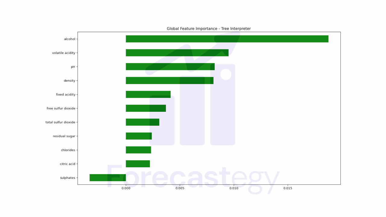
We can plot the global feature importance by averaging the contributions of each feature across all instances.
pd.Series(np.mean(contributions, axis=0), index=X_train.columns).sort_values(ascending=True).plot.barh(color='green')
Now suppose we want to know how each feature contributes to the prediction value for a specific instance to explain why the model made a certain prediction.
We can take the contributions for that instance and plot them.
prediction, bias, contributions = ti.predict(rf, X_test)

pd.Series(contributions[0], index=X_test.columns).sort_values(ascending=True).plot.barh(color='green')
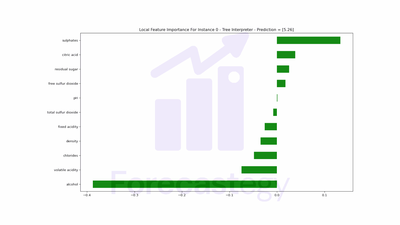
For this instance, the amount of alcohol is decreasing the prediction value, while the amount of sulphates is increasing it.
Additional Questions About Feature Importance In Random Forests
Can The Techniques Described In This Tutorial Be Applied To Classification Problems?
Yes, the techniques discussed in this tutorial can be applied to classification problems as well.
How Can I Use The Results Of The Feature Importance Analysis To Improve My Model Performance?
You can use this information to improve your model in several ways:
- Remove less important features to reduce the complexity of your model, which can help prevent overfitting and improve generalization.
- Find new features and data sources that are related to the important features.
- Try removing the most important features to check if they are really important or data leakage.
Can I Use The Same Techniques For Other Ensemble Models Like Xgboost?
Yes, you can use most of the techniques described in this tutorial for other ensemble models, such as XGBoost or LightGBM.
The concepts of feature importance, permutation importance, and handling high cardinality bias are generally applicable across different ensemble learning models.
However, the implementation details may differ depending on the specific model you are working with, so always ensure that you follow the appropriate documentation and guidelines for the model in question.
How Does Data Leakage Affect Feature Importances In Random Forests?
When data leakage occurs, information from the target variable or the test set is unintentionally incorporated into the training set, causing the model to perform exceptionally well on the training data but poorly on unseen data.
If a leaked feature is highly correlated with the target variable, the Random Forest model may assign high importance to that feature, even though it may not be genuinely predictive.
This can lead to a false sense of confidence in the model’s performance and the importance of the leaked feature.
On the other hand, as the leaked feature dominates the model’s decision-making process, other genuinely predictive features may be assigned lower importance, making it difficult to identify their true contributions to the model’s performance.
A trick I learned on Kaggle, as suggested in a previous question, is to try removing the most important features to check if they are really important or data leakage artifacts.
The rationale behind this approach is that if a feature is genuinely important, removing it should lead to a significant drop in model performance.
If removing the feature improves model performance, it’s very likely that it’s not a genuine improvement, but rather a result of data leakage.