Are you looking to make sense of your logistic regression model and determine which features are truly important in predicting your target variable?
It can be quite frustrating trying to understand which features are driving your model’s predictions, especially when you have a large number of them.
Not to mention, the presence of correlated features can make the task even more challenging.
In this tutorial, I’ll walk you through different methods for assessing feature importance in both binary and multiclass logistic regression models.
To get the most out of this tutorial, you’ll need a basic understanding of Python and fundamental machine learning concepts.
Familiarity with libraries like pandas and scikit-learn will also be helpful.
So, let’s get started!
Feature Importance In Binary Logistic Regression
The simplest way to calculate feature importance in binary logistic regression is using the model’s coefficients.
The coefficients represent the change in the log odds for a one-unit change in the predictor variable.
Larger absolute values indicate a stronger relationship between the predictor and the target variable.
Let’s load the Red Wine Quality dataset from the UCI Machine Learning Repository.
This dataset contains chemical properties of red wine as features and the quality of the wine as the target variable.
import pandas as pd
from sklearn.model_selection import train_test_split

url = "https://archive.ics.uci.edu/ml/machine-learning-databases/wine-quality/winequality-red.csv"
wine_data = pd.read_csv(url, sep=";")
wine_data['quality'] = wine_data['quality']

X = wine_data.drop('quality', axis=1)
y = wine_data['quality'].apply(lambda x: 1 if x > 5 else 0)

X_train, X_test, y_train, y_test = train_test_split(X, y, test_size=0.3, random_state=42)
| fixed acidity | volatile acidity | citric acid | residual sugar | chlorides | free sulfur dioxide | total sulfur dioxide | density | pH | sulphates | alcohol |
|---|---|---|---|---|---|---|---|---|---|---|
| 8.6 | 0.22 | 0.36 | 1.9 | 0.064 | 53 | 77 | 0.99604 | 3.47 | 0.87 | 11 |
| 12.5 | 0.46 | 0.63 | 2 | 0.071 | 6 | 15 | 0.9988 | 2.99 | 0.87 | 10.2 |
| 7.2 | 0.54 | 0.27 | 2.6 | 0.084 | 12 | 78 | 0.9964 | 3.39 | 0.71 | 11 |
| 6.4 | 0.67 | 0.08 | 2.1 | 0.045 | 19 | 48 | 0.9949 | 3.49 | 0.49 | 11.4 |
| 7.5 | 0.58 | 0.14 | 2.2 | 0.077 | 27 | 60 | 0.9963 | 3.28 | 0.59 | 9.8 |
Originally, the target variable is a continuous variable ranging from 3 to 8. I binarized it by setting the threshold to 5.
Now, let’s train a logistic regression model on the training set.
import numpy as np
import pandas as pd
from sklearn.linear_model import LogisticRegression
from sklearn.preprocessing import StandardScaler
scaler = StandardScaler()
X_train = scaler.fit_transform(X_train)
X_test = scaler.transform(X_test)
model = LogisticRegression()
model.fit(X_train, y_train)
coefficients = model.coef_[0]
feature_importance = pd.DataFrame({'Feature': X.columns, 'Importance': np.abs(coefficients)})
feature_importance = feature_importance.sort_values('Importance', ascending=True)
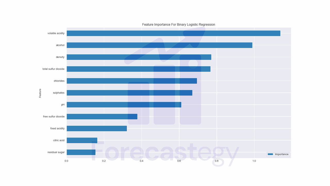
feature_importance.plot(x='Feature', y='Importance', kind='barh', figsize=(10, 6))
We first scale the features using the StandardScaler class from sklearn.preprocessing.
If the features have different scales or units, the model may give higher coefficients (thus higher importance) to the features with larger values, even if they are not necessarily more important.
For each feature, standardization subtracts the mean and divides by the standard deviation.
This makes the features have a mean of 0, a standard deviation of 1, and be approximately on the same scale.
When the features are standardized, the magnitude of the coefficients in logistic regression directly reflects the importance of each feature.
After training the model, we can access the coefficients using the coef_ attribute.
We need coef_[0] to access the model’s coefficients because the coef_ attribute returns a 2D array where each row corresponds to a class and each column corresponds to a feature.
There is only one set of coefficients for the positive class (class 1), so the coef_ attribute returns an array with a single row.
By using coef_[0], we are accessing the first (and only) row of the array, which contains the coefficients we need.

According to this method, volatile acidity, alcohol, and density are the most important features.
Let’s see how to calculate feature importance for multiclass logistic regression.
Feature Importance In Multiclass Logistic Regression
In multiclass logistic regression, we have a separate set of coefficients for each class.
We can calculate feature importance by taking the average of the absolute values of the coefficients across all classes.
Or, if we want to know the importance of a feature for a specific class, we can use the coefficients for that class.
X = wine_data.drop('quality', axis=1)
y = wine_data['quality']

X_train, X_test, y_train, y_test = train_test_split(X, y, test_size=0.3, random_state=42)
This time, we will not binarize the target variable and keep it as a multiclass problem.
Now, let’s train a logistic regression model on the training set.
import numpy as np
import pandas as pd
from sklearn.linear_model import LogisticRegression
from sklearn.preprocessing import StandardScaler
scaler = StandardScaler()
X_train = scaler.fit_transform(X_train)
X_test = scaler.transform(X_test)
model = LogisticRegression()
model.fit(X_train, y_train)
coefficients = model.coef_
avg_importance = np.mean(np.abs(coefficients), axis=0)
feature_importance = pd.DataFrame({'Feature': X.columns, 'Importance': avg_importance})
feature_importance = feature_importance.sort_values('Importance', ascending=True)
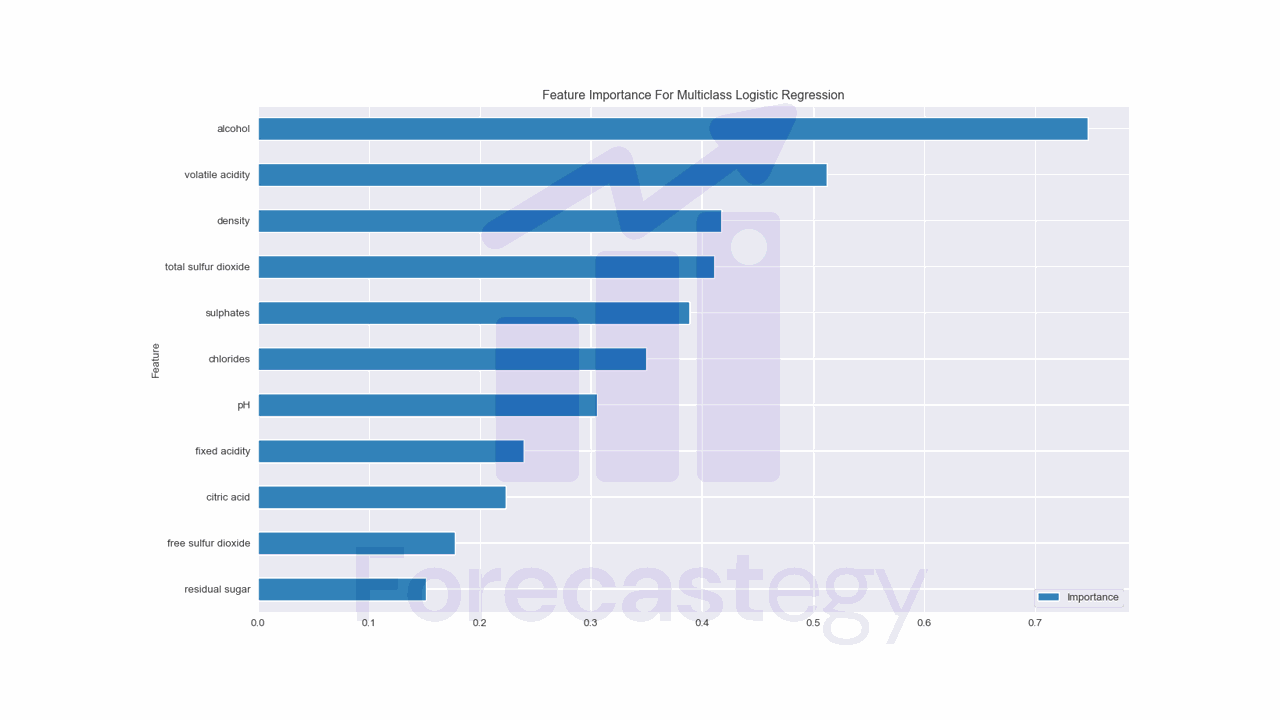
feature_importance.plot(x='Feature', y='Importance', kind='barh', figsize=(10, 6))
We first scale the features using the StandardScaler as before.
Then, we create a logistic regression model, but this time it will be a multiclass model.
After training the model, we can access the coefficients using the coef_ attribute.
Here we take the full array instead of just the first row.
We calculate the average importance across all classes by taking the mean of the absolute values of the coefficients.
These methods are simple and easy to implement, but they have some limitations.
When features are highly correlated, the coefficients can become unstable, and their magnitude might not accurately represent the actual importance of the features.
In such cases, the importance of a group of correlated features may be distributed among them, making it hard to interpret the individual importance of each feature.
Let’s try a more advanced method to calculate feature importance for logistic regression.
Permutation Importance For Logistic Regression
Permutation importance is a model-agnostic method for calculating feature importance that can be used with logistic regression.
Model-agnostic means that the method can be used with any model, not just logistic regression.
The idea behind permutation importance is to measure the drop in model performance when the values of a particular feature are shuffled randomly, after training, breaking the relationship between the feature and the target variable.
If shuffling the values of a feature results in a large drop in model performance, then the feature is important.
Scikit-learn has a built-in function for calculating permutation importance.
As this method uses the predictions in an out-of-sample dataset to calculate feature importance, we can use the model we already trained.
from sklearn.inspection import permutation_importance

result = permutation_importance(model, X_test, y_test, n_repeats=10, random_state=42)


feature_importance = pd.DataFrame({'Feature': X.columns,
                                   'Importance': result.importances_mean,
                                   'Standard Deviation': result.importances_std})
feature_importance = feature_importance.sort_values('Importance', ascending=True)


ax = feature_importance.plot(x='Feature', y='Importance', kind='barh', figsize=(10, 6), yerr='Standard Deviation', capsize=4)
ax.set_xlabel('Permutation Importance')
ax.set_title('Permutation Importance with Standard Deviation')
We need to pass the model and the validation set to the permutation_importance function.
The n_repeats parameter specifies the number of times the feature values are shuffled. More repetitions will give more accurate results, but will take longer to compute.
The random_state parameter is used to set the random seed for reproducibility.
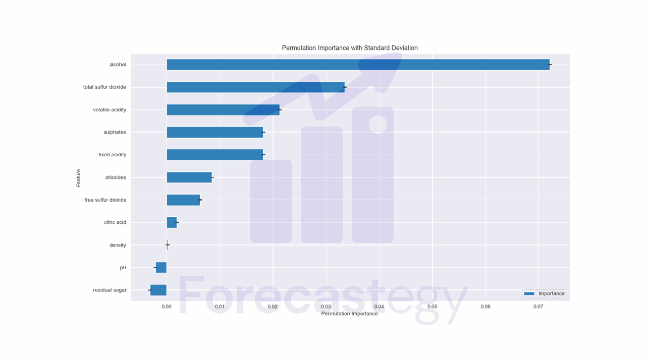
This method gives us the average importance and the standard deviation across all repetitions.
Feature Selection for Logistic Regression
While understanding feature importance is valuable, it’s often beneficial to perform explicit feature selection to reduce the dimensionality of your data and improve model performance.
Two popular techniques for feature selection, available in scikit-learn, with logistic regression are Recursive Feature Elimination (RFE) and SelectFromModel.
Recursive Feature Elimination (RFE)
Recursive Feature Elimination is a greedy optimization technique that iteratively removes the least important features from the model.
It works by fitting a base estimator (in our case, logistic regression), ranking the features based on their importance scores, and then pruning the least important features.
This process is repeated recursively until the desired number of features is reached.
from sklearn.linear_model import LogisticRegression
from sklearn.feature_selection import RFE

base_estimator = LogisticRegression()
rfe = RFE(estimator=base_estimator, n_features_to_select=5, verbose=1)
rfe.fit(X_train, y_train)

X_train_selected = rfe.transform(X_train)
X_test_selected = rfe.transform(X_test)

selected_features = X.columns[rfe.get_support()]
print(f"Selected features: {', '.join(selected_features)}")
In this example, we create a LogisticRegression instance as our base estimator and pass it to the RFE class.
The n_features_to_select parameter specifies the number of features we want to keep, and the verbose parameter controls the verbosity of the output.
After fitting the RFE object, we can use its transform method to apply the selected features to our training and test data.
The get_support method returns a boolean mask indicating which features were selected, which we can use to extract the names of the selected features.
SelectFromModel
SelectFromModel is another feature selection technique that selects features based on the importance weights calculated by an estimator.
In the case of logistic regression, it can use the model coefficients as importance weights.
from sklearn.linear_model import LogisticRegression
from sklearn.feature_selection import SelectFromModel

base_estimator = LogisticRegression()
sfm = SelectFromModel(estimator=base_estimator, threshold='median')
sfm.fit(X_train, y_train)

X_train_selected = sfm.transform(X_train)
X_test_selected = sfm.transform(X_test)

selected_features = X.columns[sfm.get_support()]
print(f"Selected features: {', '.join(selected_features)}")
Here, we create a LogisticRegression instance as our base estimator and pass it to the SelectFromModel class.
The threshold parameter determines the threshold for feature selection. In this example, we use 'median', which selects features whose importance is above the median importance of all features.
After fitting the SelectFromModel object, we can use its transform method to apply the selected features to our training and test data.
The get_support method returns a boolean mask indicating which features were selected, which we can use to extract the names of the selected features.
Both RFE and SelectFromModel can help improve model performance by reducing overfitting and improving interpretability.
However, it’s important to note that feature selection should be performed on the training data only and then applied to the test data to avoid data leakage.
You can still use the validation set to evaluate the performance of the model after feature selection without major issues, but make sure to keep the test set separate until the final evaluation.
I did not scale the data just to keep the code simple. However, it’s a good practice to do it for feature selection as well.
Additional Questions About Feature Importance In Logistic Regression
How To Handle Highly Correlated Features?
Remove or combine them.
You can either drop one of the correlated features or create a new feature that combines information from both.
How To Interpret The Negative And Positive Coefficients?
A positive coefficient means that an increase in the feature value will increase the log odds of the positive class, making it more likely.
On the other hand, a negative coefficient means that an increase in the feature value will decrease the log odds of the positive class, making it less likely.
How To Get The Feature Importance For A Specific Class In Multiclass Logistic Regression?
To calculate feature importance for a specific class, you can use the coefficients for that class.
class_index = 2  # Set the index of the class you are interested in

coefficients = model.coef_[class_index]  # Access the coefficients for the specific class

feature_importance = pd.DataFrame({'Feature': X.columns, 'Importance': np.abs(coefficients)})
feature_importance = feature_importance.sort_values('Importance', ascending=True)
feature_importance.plot(x='Feature', y='Importance', kind='barh', figsize=(1280/96, 720/96))
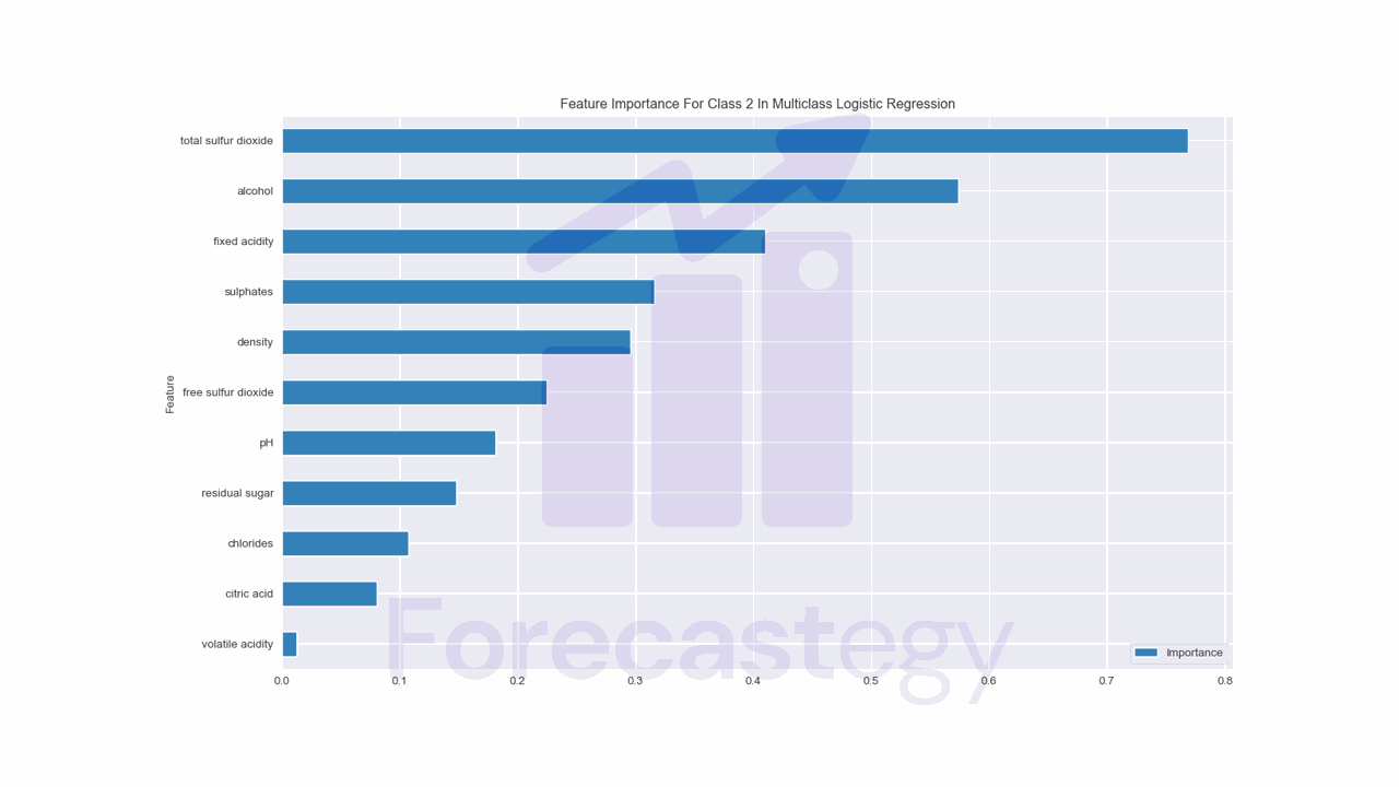
Replace class_index with the index of the class you want to analyze (e.g., 0 for the first class, 1 for the second class, and so on).
This modified code will calculate the feature importance for the specified class using its corresponding coefficients.
Check how to get feature importances from LightGBM models in the next lesson.