
LightGBM is a popular gradient boosting framework that uses tree-based learning algorithms.
These algorithms are excellent for handling tabular data and are widely used in various machine learning applications.
One of the key aspects of understanding your model’s behavior is knowing which features contribute the most to its predictions, and that’s where feature importance comes into play.
By the end of this guide, you’ll have a better grasp on the importance of your features and how to visualize them, which will help you improve your model’s performance and interpretability.
How Does LightGBM Calculate Feature Importance?
Before delving into the specific methods for calculating feature importance in LightGBM, it’s crucial to understand that there are two primary methods to do so: gain and split.
Each method looks at different aspects of the decision trees within the model to derive the importance of features. Here’s a brief overview of each method:
-
Gain: The gain method calculates feature importance based on the improvement in the splitting criterion (e.g., Gini impurity, information gain, squared error) that results from using a feature in a tree’s split. In other words, it measures how much a feature contributes to reducing the overall error or increasing the purity of nodes in the trees.
-
Split: The split method, on the other hand, calculates feature importance by counting how many times a feature is used to split nodes across all the trees in the model. This method focuses on the frequency of a feature being used in the trees, as it assumes that more frequently used features are more important.
Both methods have their assumptions and are not perfect. However, they can provide valuable insights into the features of your model.
In both cases, the higher the value, the more important the feature is.
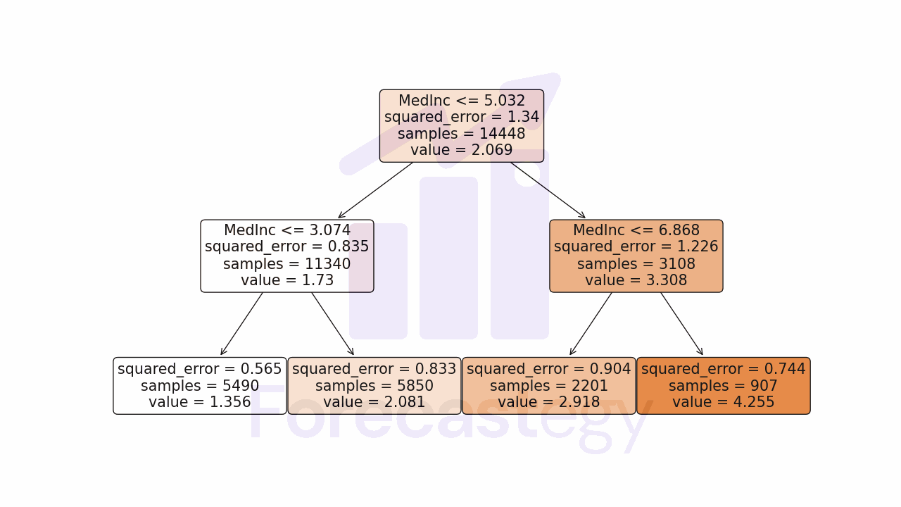
In this example decision tree, the feature ‘MedInc’ was selected in 3 splits, so it would have a split importance of 3 and all other features would have a split importance of 0.
To get the gain, you can take the difference between the squared error of the parent node and the error of the child nodes.
Compared to the root (first) node error of 1.34, the error of the leftmost child node is 0.744. A reduction of almost half.
When building the tree, no other feature was able to reduce the error as much as ‘MedInc’.
Let’s explore gain and split feature importance in more detail and provide code examples to demonstrate how to obtain them using LightGBM.
Gain Feature Importance
Let’s start by taking a closer look at the gain feature importance method.
As mentioned earlier, gain measures the improvement in the splitting criterion that results from using a feature in a tree’s split.
Imagine you’re a coach for a sports team, and you want to determine the importance of each player based on their contribution to the team’s overall score.
The players represent the features in your dataset, and their contributions represent the gain.
In this analogy, the gain is like the additional points a player contributes when they are in the game compared to when they are not.
So, if a player’s presence on the field consistently leads to higher scores or better performance, their gain would be higher, making them an important player for the team.
Similarly, in LightGBM, when a feature leads to a significant improvement in the splitting criterion (e.g., reducing the error or increasing the purity of nodes), it’s considered to have a higher gain.
Just as a more important player contributes more to the team’s performance, a feature with higher gain is more crucial for the model’s overall accuracy.
For each feature, the gain is calculated as the sum of the improvements it provides across all the trees in the model, normalized by the number of splits that included the feature. This normalization ensures a fair comparison between features.
Now, let’s see a code example to demonstrate how to obtain gain feature importance using the scikit-learn API for LightGBM:
import lightgbm as lgb
from sklearn.datasets import fetch_california_housing
from sklearn.model_selection import train_test_split
import pandas as pd

# Load dataset and split into training and testing sets
data = fetch_california_housing()
X_train, X_test, y_train, y_test = train_test_split(data.data, data.target, test_size=0.2, random_state=42)

# Train a LightGBM model
model = lgb.LGBMRegressor(importance_type='gain')
model.fit(X_train, y_train)

# Obtain gain feature importance
gain_importance = model.feature_importances_

# Display feature importance with feature names
feature_names = data.feature_names
gain_importance_df = pd.DataFrame({'Feature': feature_names, 'Gain': gain_importance})
print(gain_importance_df.sort_values(by='Gain', ascending=False))
| Feature | Gain |
|---|---|
| MedInc | 57861.9 |
| AveOccup | 13410.2 |
| Longitude | 11988.3 |
| Latitude | 10905 |
| HouseAge | 4284.05 |
| AveRooms | 2498.35 |
| AveBedrms | 895.676 |
| Population | 752.713 |
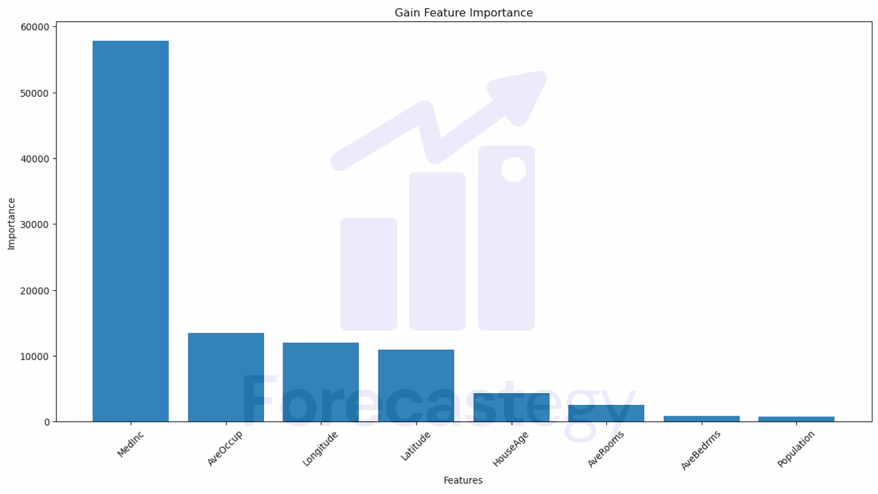
The table is sorted in descending order of gain, meaning that the features at the top contribute more to the improvement in the splitting criterion than the ones at the bottom.
‘MedInc’, which is the median income of the house’s neighborhood, with a gain of 57,861.9, has the highest importance among all features. It contributes the most to reducing error or increasing purity within the trees, and thus has a significant impact on the model’s predictions.
The process is the same for a classification problem, except you would use a classifier instead of a regressor.
Split Feature Importance
Now let’s explore the split feature importance method.
As previously mentioned, the split method calculates feature importance by counting how many times a feature is used to split nodes across all the trees in the model.
This method focuses on the frequency of a feature being used in the trees, as it assumes that more frequently used features are more important.
Think of the sports team analogy again, but this time, instead of focusing on the players’ contributions to the overall score, we’re interested in how often they participate in games.
The more a player makes the starting lineup, the more important they are for the team.
Similarly, in LightGBM, a feature that is frequently used for splitting nodes across the trees is considered to have higher split importance.
It implies that this feature plays a crucial role in the model’s decision-making process.
Now, let’s see a code example to demonstrate how to obtain split feature importance using the scikit-learn API for LightGBM:
import lightgbm as lgb
from sklearn.datasets import fetch_california_housing
from sklearn.model_selection import train_test_split
import pandas as pd

# Load dataset and split into training and testing sets
data = fetch_california_housing()
X_train, X_test, y_train, y_test = train_test_split(data.data, data.target, test_size=0.2, random_state=42)

# Train a LightGBM model
model = lgb.LGBMRegressor(importance_type='split')
model.fit(X_train, y_train)

# Obtain split feature importance
split_importance = model.feature_importances_

# Display feature importance with feature names
feature_names = data.feature_names
split_importance_df = pd.DataFrame({'Feature': feature_names, 'Split': split_importance})
print(split_importance_df.sort_values(by='Split', ascending=False))
| Feature | Split |
|---|---|
| Longitude | 686 |
| Latitude | 682 |
| MedInc | 386 |
| AveOccup | 369 |
| HouseAge | 261 |
| AveRooms | 248 |
| Population | 196 |
| AveBedrms | 172 |
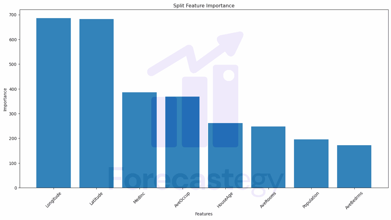
The given table displays the split feature importance for the same dataset used in the Gain table.
It is sorted in descending order of split importance, which means that the features at the top are used more frequently to split nodes in the trees compared to those at the bottom.
Comparing this table with the Gain table, we can observe some differences in the feature importances:
- ‘Longitude’ and ‘Latitude’: These two features have the highest split importance, with 686 and 682 splits respectively. This means they were used frequently for splitting nodes in the trees. However, in the Gain table, they were ranked third and fourth, indicating that although they were frequently used for splits, their individual contributions to the splitting criterion were not as high as ‘MedInc’ and ‘AveOccup’.
- ‘MedInc’: This feature was the most important in the Gain table, but it ranks third in the Split table, with 386 splits. This suggests that ‘MedInc’ has a significant impact on the splitting criterion when used, but it is not used as frequently as ‘Longitude’ and ‘Latitude’ for splitting nodes.
So, which method should you use?
How To Pick Between Gain And Split Feature Importance
As we saw in the previous examples, Gain and Split importances can yield different rankings for features.
Gain focuses on the improvement in the splitting criterion that a feature provides, whereas Split measures the frequency of a feature being used for splits in the trees.
In order to get a more comprehensive understanding of your model, you can consider comparing the results of both methods:
-
Identify overlapping important features: Features that rank high in both Gain and Split importances are likely to be truly important for your model. These features not only contribute significantly to the improvement in the splitting criterion but are also frequently used for splitting nodes.
-
Investigate discrepancies: If a feature has high importance in one method but low importance in the other, it’s worth investigating further to understand its role in your model. This can help you uncover any biases or quirks in your data or model and lead to potential improvements.
-
Artificially-inflated importances: If a feature has many different levels, it can be artificially inflated in the Split method. This is because the tree needs to split it more to find the optimal points. In this case, the Gain method is more reliable.
In practice, looking at both results and identifying where they overlap is the most reliable way I found to interpret feature importance.
Why Do Some Features Have Zero Importance In LightGBM?
LightGBM uses a leaf-wise growth strategy for decision tree construction, where it chooses the leaf with the maximum delta loss to grow.
If it can’t find an optimal split for a feature that reduces the loss, it won’t use that feature, resulting in zero feature importance.
This is reflected in both gain and split importance.
The second aspect to consider is multicollinearity, a situation where two or more features are highly correlated (which I explain in detail below).
If one feature is highly correlated with another, LightGBM may assign one a high importance and the other zero importance, in both gain and split importance.
How Does Multicollinearity Affect Feature Importance In LightGBM?
Multicollinearity occurs when two or more features in your dataset are highly correlated, causing potential issues in the interpretation of your model.
Although gradient boosting models like LightGBM are more robust to multicollinearity than linear models, it’s still essential to be aware of its presence when interpreting feature importance.
In practice, the importance will be split between the correlated features, and the sum of the importances will be equal to the importance of the original feature.
Let’s create an example using a synthetic dataset to see this effect.
We will create a dataset with three features: X1, X2, and X3, where X1 and X2 are highly correlated, and X3 is an independent feature.
import numpy as np
import pandas as pd
import lightgbm as lgb
from sklearn.model_selection import train_test_split

# Create a synthetic dataset with 1000 samples
np.random.seed(42)
n_samples = 1000

X1 = np.random.normal(0, 1, n_samples)
X2 = X1 + 0.95 * np.random.normal(0, 1, n_samples)  # Highly correlated with X1
X3 = np.random.normal(0, 1, n_samples)

X = np.column_stack((X1, X2, X3))
y = 2 * X1 + 5 * X3 + np.random.normal(0, 0.5, n_samples)  # Target variable

# Split the dataset into training and testing sets
X_train, X_test, y_train, y_test = train_test_split(X, y, test_size=0.2, random_state=42)

# Train a LightGBM model
model = lgb.LGBMRegressor(importance_type='split')
model.fit(X_train, y_train)

# Obtain split feature importance
split_importance = model.feature_importances_

# Display feature importance
feature_names = ['X1', 'X2', 'X3']
split_importance_df = pd.DataFrame({'Feature': feature_names, 'Split': split_importance})
print(split_importance_df.sort_values(by='Split', ascending=False))
| Feature | Split |
|---|---|
| X1 | 1132 |
| X3 | 1063 |
| X2 | 776 |
In this example, X1 and X2 are highly correlated features, and X3 is an independent feature.
The target variable y is a linear combination of X1 and X3.
After training the LightGBM model, you may observe that the split feature importances of X1 and X2 are close.
This result indicates that the model is splitting the importance between the correlated features, X1 and X2.
If we remove X2 from the dataset and retrain the model, we get the following results:
| Feature | Split |
|---|---|
| X1 | 1583 |
| X3 | 1391 |
Keep in mind that this is a simplified example, and in real-world datasets, the relationship between features and the target variable may be more complex.
Plotting LightGBM Feature Importance in Python
Visualizing feature importance can help make it easier to interpret and communicate your model’s behavior.
Let’s assume you have already calculated both Gain and Split feature importances, as demonstrated in previous sections.
Now, we’ll create bar plots to visualize the importances:
import matplotlib.pyplot as plt

def plot_feature_importance(importance_values, feature_names, title):
    # Create a DataFrame with feature names and importance values
    importance_df = pd.DataFrame({'Feature': feature_names, 'Importance': importance_values})
    importance_df = importance_df.sort_values(by='Importance', ascending=False)

    # Plot the feature importances
    plt.figure(figsize=(10, 6))
    plt.bar(importance_df['Feature'], importance_df['Importance'])
    plt.xlabel('Features')
    plt.ylabel('Importance')
    plt.title(title)
    plt.xticks(rotation=45)
    plt.show()

# Plot Gain feature importance
plot_feature_importance(gain_importance, feature_names, 'Gain Feature Importance')

# Plot Split feature importance
plot_feature_importance(split_importance, feature_names, 'Split Feature Importance')
This code snippet defines a function, plot_feature_importance, that takes the importance values, feature names, and a title as input, and creates a bar plot to visualize the feature importances.
The gain_importance and split_importance variables should be the outputs obtained from the previous sections.
Next, check how to get feature importances from Logistic Regression.