
Logistic regression is a type of predictive model used in machine learning and statistics.
Its purpose is to determine the likelihood of an outcome based on one or more input variables, also known as features.
For example, logistic regression can be used to predict the probability of a customer churning, given their past interactions and demographic information.
Difference Between Linear And Logistic Regression?
Before diving into logistic regression, it’s important to understand its sibling model, linear regression.
Linear regression is a predictive model that estimates a continuous value based on one or more independent variables.
For instance, it can be used to predict the price of a house based on its size and location.
The main difference between linear and logistic regression lies in the type of outcome they predict.
While linear regression predicts a continuous value, logistic regression predicts the probability of an event occurring.
In other words, linear regression is used when the dependent variable is continuous, and logistic regression is used when the dependent variable is categorical (e.g., binary classification).
An example of a binary classification problem is predicting if an email is spam or not.
As a rule of thumb, you should use linear regression when you want to predict a numerical value, and logistic regression when you want to predict the likelihood of an event happening.
Both are supervised learning algorithms.
Logistic Regression Formula
The formula for logistic regression is derived from the logistic function, also known as the sigmoid function, which is used to model the probability of a certain class or event.
The logistic function has an “S” shape and ranges from 0 to 1.
It can be defined as:
$$ p(x) = \frac{1}{1 + e^{-(b_0 + b_1 x)}} $$
where:
- $p(x)$ is the probability of the outcome (the predicted value)
- $x$ is the input feature (independent variable)
- $b_0$ is the bias term (intercept)
- $b_1$ is the coefficient (weight) assigned to the input feature $x$
In the case of multiple input features, the formula for logistic regression can be generalized as:
$$ p(x) = \frac{1}{1 + e^{-(b_0 + \sum_{i=1}^{n} b_i x_i)}} $$
where:
- $n$ is the number of input features
- $x_i$ represents the input features (independent variables)
- $b_i$ are the coefficients (weights) assigned to each input feature
Once these parameters are estimated, you can plug in the input feature values into the logistic regression formula to obtain the probability of the positive class.
To make a final classification decision, a threshold value is applied to the probability. If the probability is greater than the threshold (typically 0.5), the positive class is predicted; otherwise, the negative class is predicted.
Data Pre-processing
Before applying logistic regression, it’s essential to apply a few preprocessing steps to your data to ensure the model performs optimally.
Two key steps in preparing data for logistic regression are scaling numerical features and handling categorical features.
Scaling Numerical Features
Feature scaling is an important step in preparing your data for logistic regression because it helps to prevent features with larger values from dominating the model and even hurting convergence.
Standardization is a common method of scaling that involves transforming each feature so that it has a mean of 0 and a standard deviation of 1.
To apply standardization using sklearn’s StandardScaler, follow these steps:
- Import the
StandardScalerclass fromsklearn.preprocessing. - Create an instance of the
StandardScalerclass. - Fit the scaler to your training data using the
.fit()method. - Transform both your training and testing data using the
.transform()method.
Here’s some example code:
from sklearn.preprocessing import StandardScaler

# Instantiate the scaler
scaler = StandardScaler()

# Fit the scaler to the training data
scaler.fit(X_train)

# Transform the training and testing data
X_train_scaled = scaler.transform(X_train)
X_test_scaled = scaler.transform(X_test)
Always split your data into training and testing sets BEFORE applying feature scaling or you’ll risk data leakage.
Handling Categorical Features With One-Hot Encoding
Logistic regression works with numerical input variables.
However, datasets often have categorical features that need to be converted into a numerical format before using them in a logistic regression model.
One way to do this is by using one-hot encoding.
In this example, we’ll use the category_encoders library to apply one-hot encoding to a dataframe.
This library has many other useful encoders for handling categorical features, such as target encoding and binary encoding.
To apply one-hot encoding using the category_encoders library, follow these steps:
-
Import the
OneHotEncoderclass fromcategory_encoders. -
Make a list of the categorical columns in the dataframe.
-
Instantiate the
OneHotEncoderclass, specifying the categorical columns and settinguse_cat_names=Trueto keep the original category names in the encoded features. -
Use the
.fit_transform()method on the dataframe to apply one-hot encoding and get the transformed data.
Here’s the example code:
import numpy as np
import pandas as pd
from category_encoders import OneHotEncoder
from sklearn.model_selection import train_test_split

df = pd.DataFrame({
    'numerical': np.random.randn(100),
    'categorical1': np.random.choice(['A', 'B', 'C'], size=100),
    'categorical2': np.random.choice(['X', 'Y', 'Z'], size=100),
    'categorical3': np.random.choice(['M', 'N', 'O'], size=100),
    'target': np.random.choice([0, 1], size=100)
})

X = df.drop('target', axis=1)
y = df['target']

X_train, X_test, y_train, y_test = train_test_split(X, y, test_size=0.2, random_state=42)

categorical_columns = ['categorical1', 'categorical2', 'categorical3']

encoder = OneHotEncoder(cols=categorical_columns, use_cat_names=True)

transformed_train_data = encoder.fit_transform(X_train)
transformed_test_data = encoder.transform(X_test)
| numerical | categorical1_C | categorical1_A | categorical1_B | categorical2_Z | categorical2_X | categorical2_Y | categorical3_O | categorical3_M | categorical3_N |
|---|---|---|---|---|---|---|---|---|---|
| 0.603863 | 1 | 0 | 0 | 1 | 0 | 0 | 1 | 0 | 0 |
| -0.746848 | 1 | 0 | 0 | 0 | 1 | 0 | 1 | 0 | 0 |
| 0.316617 | 1 | 0 | 0 | 0 | 1 | 0 | 1 | 0 | 0 |
| 0.430625 | 0 | 1 | 0 | 1 | 0 | 0 | 0 | 1 | 0 |
| 0.642965 | 1 | 0 | 0 | 1 | 0 | 0 | 0 | 1 | 0 |
As shown above, the categorical features have been converted into numerical features using one-hot encoding.
category_encoders returns a dataframe with the transformed data plus the original columns, which makes it easy to continue working with the data.
This is why I prefer it over sklearn.preprocessing.OneHotEncoder.
Now that you understand how to prepare your data for logistic regression, let’s take a look at how to apply it in Python in a real dataset.
Logistic Regression For Binary Classification Using Scikit-Learn
Binary classification involves predicting one of two possible outcomes.
In this code, we are building a logistic regression model to predict credit risk (good or bad) based on various input features.
We’ll go through the process step by step.
First, we import the necessary libraries, including sklearn and category_encoders.
import pandas as pd
from sklearn.model_selection import train_test_split
from sklearn.linear_model import LogisticRegression
from sklearn.metrics import accuracy_score
from sklearn.datasets import fetch_openml
from sklearn.preprocessing import StandardScaler
from category_encoders import OneHotEncoder
We load the “credit-g” dataset from the OpenML repository, which contains credit risk data.
# Load the dataset
data = fetch_openml('credit-g', version=1, as_frame=True)
X = data.data
y = data.target
| checking_status | duration | credit_history | purpose | credit_amount | savings_status | employment | installment_commitment | personal_status | other_parties | residence_since | property_magnitude | age | other_payment_plans | housing | existing_credits | job | num_dependents | own_telephone | foreign_worker |
|---|---|---|---|---|---|---|---|---|---|---|---|---|---|---|---|---|---|---|---|
| <0 | 6 | critical/other existing credit | radio/tv | 1169 | no known savings | >=7 | 4 | male single | none | 4 | real estate | 67 | none | own | 2 | skilled | 1 | yes | yes |
| 0<=X<200 | 48 | existing paid | radio/tv | 5951 | <100 | 1<=X<4 | 2 | female div/dep/mar | none | 2 | real estate | 22 | none | own | 1 | skilled | 1 | none | yes |
| no checking | 12 | critical/other existing credit | education | 2096 | <100 | 4<=X<7 | 2 | male single | none | 3 | real estate | 49 | none | own | 1 | unskilled resident | 2 | none | yes |
| <0 | 42 | existing paid | furniture/equipment | 7882 | <100 | 4<=X<7 | 2 | male single | guarantor | 4 | life insurance | 45 | none | for free | 1 | skilled | 2 | none | yes |
| <0 | 24 | delayed previously | new car | 4870 | <100 | 1<=X<4 | 3 | male single | none | 4 | no known property | 53 | none | for free | 2 | skilled | 2 | none | yes |
We separate the dataset into input features (X) and the target variable (y).
The input features consist of both categorical and numerical variables that will be used to predict the credit risk.
The target variable is the credit risk classification (“good” or “bad”).
To evaluate our model’s performance, we need to split the dataset into a training set and a testing set.
We use the train_test_split() function to allocate 80% of the data for training and 20% for testing.
# Split the dataset into training and testing sets
X_train, X_test, y_train, y_test = train_test_split(X, y, test_size=0.2, random_state=42)
Like explained above, before we can use the data to train our model, we need to preprocess it.
We start by identifying the categorical and numerical columns in our dataset.
Next, we apply one-hot encoding to the categorical columns using the OneHotEncoder class from category_encoders.
This converts the categorical variables into a binary format that our model can understand.
We then scale the numerical columns using the StandardScaler class from sklearn to ensure that all features have a similar range of values.
# Preprocess the data
category_names = X_train.select_dtypes(include='category').columns
numeric_names = X_train.select_dtypes(include='number').columns

ohe = OneHotEncoder(cols=category_names, use_cat_names=True)
X_train = ohe.fit_transform(X_train)
X_test = ohe.transform(X_test)

scaler = StandardScaler()
X_train.loc[:, numeric_names] = scaler.fit_transform(X_train.loc[:, numeric_names])
X_test.loc[:, numeric_names] = scaler.transform(X_test.loc[:, numeric_names])
Notice the difference between the training and testing data: we use fit_transform() on the training data and transform() on the testing data.
transform() applies the same transformations to the testing data as the training data, while fit_transform() has an additional step of fitting the preprocessing parameters on the training data.
In the case of StandardScaler, the parameters are the mean and standard deviation of each column.
If you use fit_transform() on the testing data, you will leak information from the testing data into the training process, as you don’t know the mean and standard deviation of the testing data in real life.
Now that our data is prepared, we can build the logistic regression model.
We create an instance of the LogisticRegression class and fit it to the preprocessed training data.
# Instantiate the logistic regression model
log_reg = LogisticRegression()

# Fit the model to the training data
log_reg.fit(X_train, y_train)
With our model trained, it’s time to see how well it performs on unseen data.
We use the model to make predictions on the preprocessed testing data.
# Predict the outcomes for the testing data
y_pred = log_reg.predict(X_test)

# Evaluate the model's performance
accuracy = accuracy_score(y_test, y_pred)
print("Accuracy:", accuracy)
To determine how well our model is performing, we compare its predictions to the true outcomes in the testing set.
We use the accuracy_score() function from sklearn to calculate the accuracy of our model.
Finally, we print the accuracy score, which tells us how accurately our model is predicting credit risk.
Multinomial Logistic Regression For Multi-Class Classification Using Scikit-Learn
Multi-class classification involves predicting one of multiple possible outcomes.
In this code, we are building a multinomial logistic regression model to predict the age of abalone based on various input features.
Abalone is a type of shellfish that is commonly found in the ocean.
This could be set up as a regression problem, but the dataset is usually treated as a classification problem.
We have 28 classes corresponding to the number of rings in the abalone shell, which is a good indicator of age.
First, we import the necessary libraries.
import pandas as pd
from sklearn.model_selection import train_test_split
from sklearn.linear_model import LogisticRegression
from sklearn.metrics import accuracy_score
from sklearn.datasets import fetch_openml
from sklearn.preprocessing import StandardScaler
We load the “abalone” dataset from the OpenML repository, which contains abalone age data.
# Load the dataset
data = fetch_openml('abalone', version=1, as_frame=True)
X = data.data
y = data.target
We separate the dataset into input features (X) and the target variable (y).
The input features consist of both categorical and numerical variables that will be used to predict the abalone age.
The target variable is split into 28 classes corresponding to the number of rings in the abalone shell.
To evaluate our model’s performance, we need to split the dataset into a training set and a testing set.
We use the train_test_split() function to allocate 80% of the data for training and 20% for testing.
# Split the dataset into training and testing sets
X_train, X_test, y_train, y_test = train_test_split(X, y, test_size=0.2, random_state=42)
To preprocess the data, we start by identifying the categorical and numerical columns in our dataset.
We apply one-hot encoding to the categorical columns using the OneHotEncoder class from category_encoders.
Next, we scale the numerical columns using the StandardScaler class from sklearn to ensure that all features have a similar range of values.
# Preprocess the data
category_names = X_train.select_dtypes(include='category').columns
numeric_names = X_train.select_dtypes(include='number').columns

ohe = OneHotEncoder(cols=category_names, use_cat_names=True)
X_train = ohe.fit_transform(X_train)
X_test = ohe.transform(X_test)

scaler = StandardScaler()
X_train.loc[:, numeric_names] = scaler.fit_transform(X_train.loc[:, numeric_names])
X_test.loc[:, numeric_names] = scaler.transform(X_test.loc[:, numeric_names])
Now that our data is prepared, we can build the logistic regression model.
We create an instance of the LogisticRegression class, specify we want it to use the multinomial mode, and fit it to the preprocessed training data.
# Instantiate the logistic regression model
log_reg = LogisticRegression(multi_class='multinomial')

# Fit the model to the training data
log_reg.fit(X_train, y_train)
With our model trained, it’s time to see how well it performs on unseen data.
We use the model to make predictions on the preprocessed testing data.
# Predict the outcomes for the testing data
y_pred = log_reg.predict(X_test)

# Evaluate the model's performance
accuracy = accuracy_score(y_test, y_pred)
print("Accuracy:", accuracy)
To determine how well our model is performing, we compare its predictions to the true outcomes in the testing set with the accuracy_score() function from sklearn.
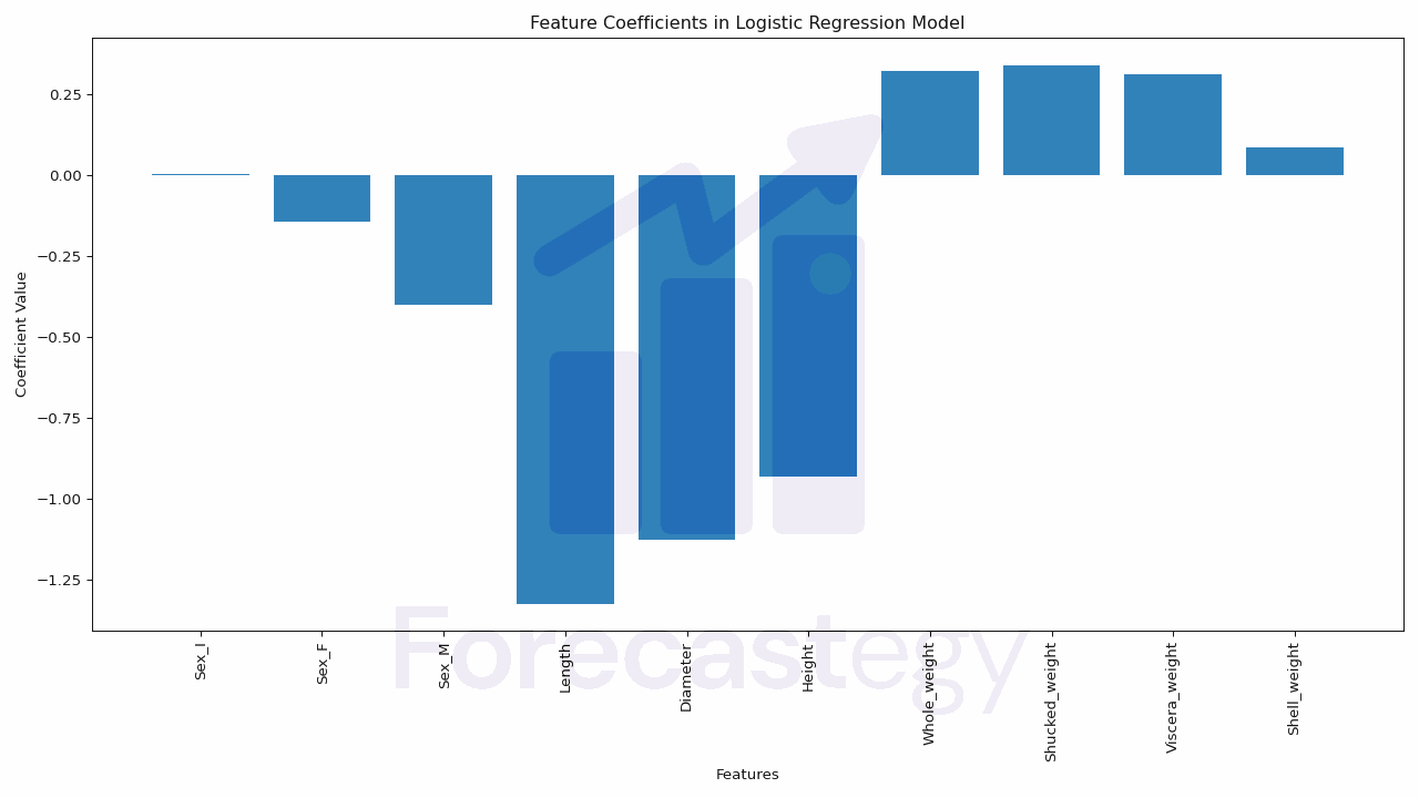
Extracting Coefficients From A Scikit-learn Logistic Regression Model
The coefficients in a logistic regression model represent the relationship between the input features and the predicted outcome.
They indicate the importance and influence of each feature on the prediction.
In this section, you’ll learn how to access and analyze the coefficients and intercept of our trained logistic regression model using scikit-learn.
The coef_ attribute of the trained logistic regression model gives us the coefficients, while the intercept_ attribute provides the model’s intercept.
Here’s a code example to demonstrate how to access and display the coefficients and intercept:
# Import necessary libraries
from sklearn.linear_model import LogisticRegression

# Assuming `X_train` and `y_train` are the preprocessed training data
# Instantiate and train the logistic regression model
log_reg = LogisticRegression()
log_reg.fit(X_train, y_train)

# Access the coefficients and intercept
coefficients = log_reg.coef_
intercept = log_reg.intercept_

# Display the coefficients and intercept
print("Coefficients:")
print(coefficients)
print("\nIntercept:")
print(intercept)
In the output, you’ll see the coefficients for each input feature along with the intercept.
If the coefficient is positive, it means that the feature has a positive influence on the predicted outcome.
Conversely, if the coefficient is negative, the feature has a negative influence.
The magnitude of the coefficient indicates the strength of the relationship between the feature and the prediction.
In the case of multi-class classification, the coefficients and intercepts are structured differently compared to binary classification.
The coef_ attribute will contain an array with multiple rows, where each row represents the coefficients for a specific class.
Similarly, the intercept_ attribute will contain multiple values, one for each class.
How To Get The Predicted Probabilities From Logistic Regression In Scikit-learn
In logistic regression, we’re not only interested in the predicted class itself, but also the probability of an input belonging to each class.
Predicted probabilities can be useful when you want to make decisions based on the confidence level of the predictions.
Scikit-learn’s logistic regression model offers a method called predict_proba() to obtain the predicted probabilities for each class.
In this section, we’ll demonstrate how to use this method on test data and interpret the output.
Assuming you have a trained logistic regression model log_reg and preprocessed test data X_test, you can get the predicted probabilities as follows:
predicted_probabilities = log_reg.predict_proba(X_test)
The output predicted_probabilities is a NumPy array with shape (n_samples, n_classes), where n_samples is the number of samples in the test data and n_classes is the number of classes in the target variable.
Each row in this array contains the predicted probabilities for each class.
For example, if we have a multi-class classification problem with 3 classes (A, B, and C), the output might look like this:
array([[0.1, 0.8, 0.1],
       [0.3, 0.4, 0.3],
       [0.9, 0.05, 0.05],
       ...,
       [0.2, 0.3, 0.5]])
In this example, the first row represents the predicted probabilities for the first sample in the test data: 10% chance of belonging to class A, 80% chance of belonging to class B, and 10% chance of belonging to class C.
In the binary case, it outputs a 2D array with shape (n_samples, 2), where the first column contains the predicted probabilities for the negative class and the second column contains the predicted probabilities for the positive class.
To extract the probabilities for a specific class, you can use array slicing.
For instance, if you want to get the predicted probabilities for class B, you can do the following:
class_B_probabilities = predicted_probabilities[:, 1]
This will give you an array of probabilities for class B for all samples in the test data.
Hyperparameter Tuning With Grid Search And Cross-Validation
In our logistic regression model, we have various hyperparameters that can be adjusted to optimize the model’s performance.
In this section, we will focus on tuning two key hyperparameters: C and penalty.
C is the inverse of regularization strength. Smaller values of C result in stronger regularization, which can help prevent overfitting. However, too much regularization might lead to underfitting.
penalty determines the type of regularization applied to the model. In scikit-learn’s logistic regression, the options are 'l1', 'l2', 'elasticnet', and 'none'.
To tune these hyperparameters, we will use GridSearchCV from scikit-learn.
This will perform an exhaustive search over a specified parameter grid and determine the best combination of hyperparameter values for our model.
I am a big proponent of more advanced hyperparameter tuning methods such as Bayesian optimization and random search when we have many hyperparameters to tune.
Here, we have only two, so a simple grid search will suffice.
Let’s see how to perform this search.
Import the necessary libraries.
from sklearn.model_selection import GridSearchCV
Set up the hyperparameter grid.
param_grid = {
    'C': [0.001, 0.01, 0.1, 1, 10, 100],
    'penalty': ['l1', 'l2', 'elasticnet', 'none']
}
This will create a grid with 24 combinations of hyperparameter values: 6 values for C multiplied by 4 values for penalty equals 24 combinations.
Instantiate the logistic regression model with the multi_class='multinomial' parameter.
log_reg = LogisticRegression(multi_class='multinomial')
The same method can be used with binary classification, but here I am keeping up with the multi-class classification example.
Create the GridSearchCV object, passing in the logistic regression model, hyperparameter grid, and a scoring metric (e.g., accuracy):
grid_search = GridSearchCV(log_reg, param_grid, scoring='accuracy', cv=5)
cv is the number of folds in cross-validation.
Fit the GridSearchCV object to the training data:
grid_search.fit(X_train, y_train)
Obtain the best hyperparameters and the corresponding best score:
best_params = grid_search.best_params_
best_score = grid_search.best_score_
print("Best hyperparameters:", best_params)
print("Best accuracy:", best_score)
After finishing the search, GridSearchCV, by default, retrains the logistic regression model with the best hyperparameters on the entire training set and stores it in the best_estimator_ attribute.
We can take it and use it to make predictions on the test set:
best_log_reg = grid_search.best_estimator_
y_pred = best_log_reg.predict(X_test)
accuracy = accuracy_score(y_test, y_pred)
print("Accuracy with best hyperparameters:", accuracy)
Dealing With Class Imbalance With Class Weights
Class imbalance occurs when one class has significantly more samples than another.
For example, when classifying spam emails, you might have 99% of the data belonging to the negative class (not spam) and only 1% belonging to the positive class (spam).
This can lead to a biased model that performs poorly on the underrepresented class.
To deal with class imbalance in logistic regression, you can use the class_weight parameter in sklearn’s LogisticRegression class.
This is the best way, by far, that I found in practice. It beats any other method I tried, including oversampling and undersampling.
You can set class_weight to 'balanced' to automatically adjust the weights based on the number of samples in each class:
# Instantiate the logistic regression model with balanced class weights
log_reg_balanced = LogisticRegression(class_weight='balanced')

# Fit the model to the training data
log_reg_balanced.fit(X_train, y_train)

# Predict the outcomes for the testing data
y_pred_balanced = log_reg_balanced.predict(X_test)
According to sklearn’s documentation, this will set the weights to n_samples / (n_classes * np.bincount(y)).
Let’s say we have a dataset with two classes, A and B, and the following counts:
- Class A: 20 samples
- Class B: 80 samples
np.bincount(y) calculates the number of occurrences of each class label in the dataset y. In our example, the bincount would be [20, 80].
n_classes is the number of distinct classes in the dataset. In our example, we have two classes (A and B), so n_classes = 2.
n_samples is the total number of samples in the dataset. In our example, there are 100 samples (20 from class A and 80 from class B).
Alternatively, you can provide a dictionary specifying custom weights for each class:
# Define custom class weights
class_weights = {0: 1, 1: 5}

# Instantiate the logistic regression model with custom class weights
log_reg_custom = LogisticRegression(class_weight=class_weights)

# Fit the model to the training data
log_reg_custom.fit(X_train, y_train)

# Predict the outcomes for the testing data
y_pred_custom = log_reg_custom.predict(X_test)