
As a Python user aiming to predict a continuous target variable from a dataset with both numerical and categorical features, you’ve made a great choice in considering CatBoost.
This high-performance machine learning algorithm is particularly known for its ability to handle categorical variables effectively.
In this tutorial, I’ll guide you step-by-step on how to use CatBoost for regression tasks.
We’ll start from preparing your data, training the CatBoost model, and finally evaluating its performance.
By the end of this tutorial, you’ll have a solid understanding of how to use CatBoost for regression tasks in Python.
Regression Objective Function In CatBoost
Different than classification, in regression tasks we are trying to predict a continuous value, such as the price of a house or the number of sales of a product.
Because of that, the loss function we commonly use is the Mean Squared Error (MSE).
The MSE calculates the average squared difference between the actual and predicted values. It’s a popular choice because it punishes larger errors more than smaller ones.
That said, CatBoost can optimize a variety of loss functions, including the MAE, Poisson and Quantile.
Installing CatBoost in Python
Installing CatBoost in your Python environment is straightforward and can be done using either pip or conda.
To install CatBoost using pip, you can use the following command in your terminal:
pip install catboost
If you prefer using conda, you can install CatBoost with the following command:
conda install -c conda-forge catboost
Remember to run these commands in your terminal, not in your Python script or notebook.
Once the installation is complete, you can import CatBoost into your Python script using:
import catboost
This will allow you to access all the functionalities of CatBoost in your script.
Loading and Preprocessing Data
Before we can start training our model, we need to load and preprocess our data.
We’ll be using the Melbourne Housing Snapshot Dataset for this tutorial.
This dataset contains both numerical and categorical features of houses in Melbourne, Australia, and the goal is to predict the price of a house.
First, let’s load the dataset using Pandas. We’ll use the read_csv() function, which allows us to read a CSV file and load it into a DataFrame.
import pandas as pd

data = pd.read_csv('melb_data.csv')
After loading the data, it’s a good practice to look at the first few rows using the head() function. This will give you a quick overview of the data you’ll be working with.
data.head()
| Suburb | Address | Rooms | Type | Price | Method | SellerG | Date | Distance | Postcode | Bedroom2 | Bathroom | Car | Landsize | BuildingArea | YearBuilt | CouncilArea | Lattitude | Longtitude | Regionname | Propertycount | |
|---|---|---|---|---|---|---|---|---|---|---|---|---|---|---|---|---|---|---|---|---|---|
| 0 | Abbotsford | 85 Turner St | 2 | h | 1.48e+06 | S | Biggin | 3/12/2016 | 2.5 | 3067 | 2 | 1 | 1 | 202 | nan | nan | Yarra | -37.7996 | 144.998 | Northern Metropolitan | 4019 |
| 1 | Abbotsford | 25 Bloomburg St | 2 | h | 1.035e+06 | S | Biggin | 4/02/2016 | 2.5 | 3067 | 2 | 1 | 0 | 156 | 79 | 1900 | Yarra | -37.8079 | 144.993 | Northern Metropolitan | 4019 |
| 2 | Abbotsford | 5 Charles St | 3 | h | 1.465e+06 | SP | Biggin | 4/03/2017 | 2.5 | 3067 | 3 | 2 | 0 | 134 | 150 | 1900 | Yarra | -37.8093 | 144.994 | Northern Metropolitan | 4019 |
| 3 | Abbotsford | 40 Federation La | 3 | h | 850000 | PI | Biggin | 4/03/2017 | 2.5 | 3067 | 3 | 2 | 1 | 94 | nan | nan | Yarra | -37.7969 | 144.997 | Northern Metropolitan | 4019 |
| 4 | Abbotsford | 55a Park St | 4 | h | 1.6e+06 | VB | Nelson | 4/06/2016 | 2.5 | 3067 | 3 | 1 | 2 | 120 | 142 | 2014 | Yarra | -37.8072 | 144.994 | Northern Metropolitan | 4019 |
Now that our data is ready, we can split it into a training set and a testing set.
The training set is used to train the model, while the testing set is used to evaluate its performance.
We’ll use the train_test_split() function from the sklearn.model_selection module to do this.
from sklearn.model_selection import train_test_split

X = data.drop('Price', axis=1)
y = data['Price']

X_train, X_test, y_train, y_test = train_test_split(X, y, test_size=0.2, random_state=42)
In this code, test_size=0.2 means that 20% of the data will be used for the test set, and the rest for the training set.
random_state=42 is used to ensure that the splits you generate are reproducible. If you run the code again, you’ll get the same train/test split.
Next, we need to handle categorical variables.
CatBoost can handle categorical variables directly, but we need to specify the name of these features.
To do this, we can use the cat_features parameter and pass in a list of strings.
Let’s create this list by selecting all the columns with the object data type.
cat_features = X_train.select_dtypes(include='object').columns.tolist()

for feature in cat_features:
    X_train[feature] = X_train[feature].astype('str')
    X_test[feature] = X_test[feature].astype('str')
I added a loop to make them all strings, because otherwise CatBoost will complain that it has NaNs in the column.
You can put any value you want for the missing values, which can be even a “NaN” string, as long as your column is made of strings.
By default, any categorical feature with less than 255 unique values will be one-hot encoded. Others will be encoded with more advanced methods.
Training the CatBoost Regressor Model
Now that we have our data ready, let’s set up the CatBoost regressor model.
First, we import the necessary module from the CatBoost library.
Then, we create an instance of the CatBoostRegressor class.
When setting up the model, you can specify various hyperparameters. Here are a few key ones:
-
Learning Rate: This controls the step size at each iteration while moving toward a minimum of a loss function. A smaller learning rate requires more iterations, but can lead to a more accurate model. Conversely, a larger learning rate requires fewer iterations, but the model may be less accurate.
-
Number of Trees: This is the number of trees to be constructed in the boosting process.
-
Tree Depth: This is the depth of the trees, i.e., the maximum number of levels in each decision tree. A larger depth can make the model more complex and potentially lead to overfitting, while a smaller depth might result in underfitting. You can think about it as a regularization parameter.
Lastly, we pass the list with the names of the categorical features to the cat_features parameter.
from catboost import CatBoostRegressor

model = CatBoostRegressor(learning_rate=0.1, n_estimators=100, depth=7, cat_features=cat_features)
Once the model is set up, we can fit it to our training data using the fit() function.
model.fit(X_train, y_train)
During the training process, CatBoost displays the iteration number and the loss function value at each step.
This information can help you understand how your model is learning from the data.
If the loss function value is decreasing, it means that the model is improving.
If it’s increasing or fluctuating, it might mean that the model is struggling to learn from the data.
But be careful, because the loss function value is calculated on the training data, so it’s not a good indicator of how well your model will perform on unseen data.
Evaluating the CatBoost Regressor Model
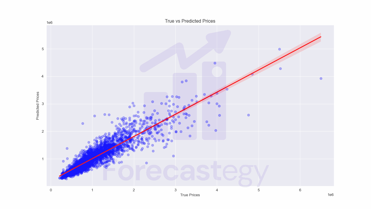
After training our model, we need to evaluate its performance on unseen data.
We do this by making predictions on our test set and comparing these predictions to the actual values.
To make predictions with our trained model, we use the predict() function and pass in our test data.
predictions = model.predict(X_test)
Now, we need to calculate some performance metrics to quantify how well our model is doing.
Two commonly used metrics for regression tasks are the Root Mean Squared Error (RMSE) and the Mean Absolute Error (MAE).
-
RMSE: This is the square root of the average of the squared differences between the actual and predicted values. It’s useful because it punishes larger errors more than smaller ones.
-
MAE: This is the average of the absolute differences between the actual and predicted values. It’s less sensitive to outliers than the RMSE.
We can calculate these metrics using the mean_squared_error and mean_absolute_error functions from the sklearn.metrics module.
from sklearn.metrics import mean_squared_error, mean_absolute_error

rmse = mean_squared_error(y_test, predictions, squared=False)
mae = mean_absolute_error(y_test, predictions)
In this code, squared=False is used to get the RMSE. If squared=True, the function returns the Mean Squared Error instead.
Remember, lower values for both RMSE and MAE indicate a better fit of the model.
These metrics provide a quantitative measure of how accurate our model’s predictions are, which can guide us in further tuning and improving it.