Last time, I learned it’s very important to have the most granular data possible to build a modern marketing mix model.
Usually, this means having daily impressions and conversions (e.g. sales) data.
I wanted to find a way to use the power of daily models even with products that don’t sell every day.
My course sales data have more days without sales than days with sales, which makes it into a zero vs something prediction instead of a regular regression.
Statistics call it zero-inflated data, and it’s quite a challenge to forecast.
After thinking about it for a while…
I Borrowed An Idea From My Quant Finance Friends
In all my readings, I haven’t found a marketing mix model that uses more than 1 non-overlapping day/week of sales as a target (dependent variable).
Although not sure why this is the case, I have a few hypotheses:
- It didn’t make sense to do it when it was only used for offline channels and sales.
- Statisticians didn’t want to break (even more) the independence assumptions about the data.
One easy trick to make models behave well in the noisy world of quant finance is trying to predict where the price will be in a given time window.
It helps to capture the underlying real price movement that we expect to happen even if the path to reach it looks like a random walk.
It got me thinking: what would happen if I try to predict sales for more than a day at a time?
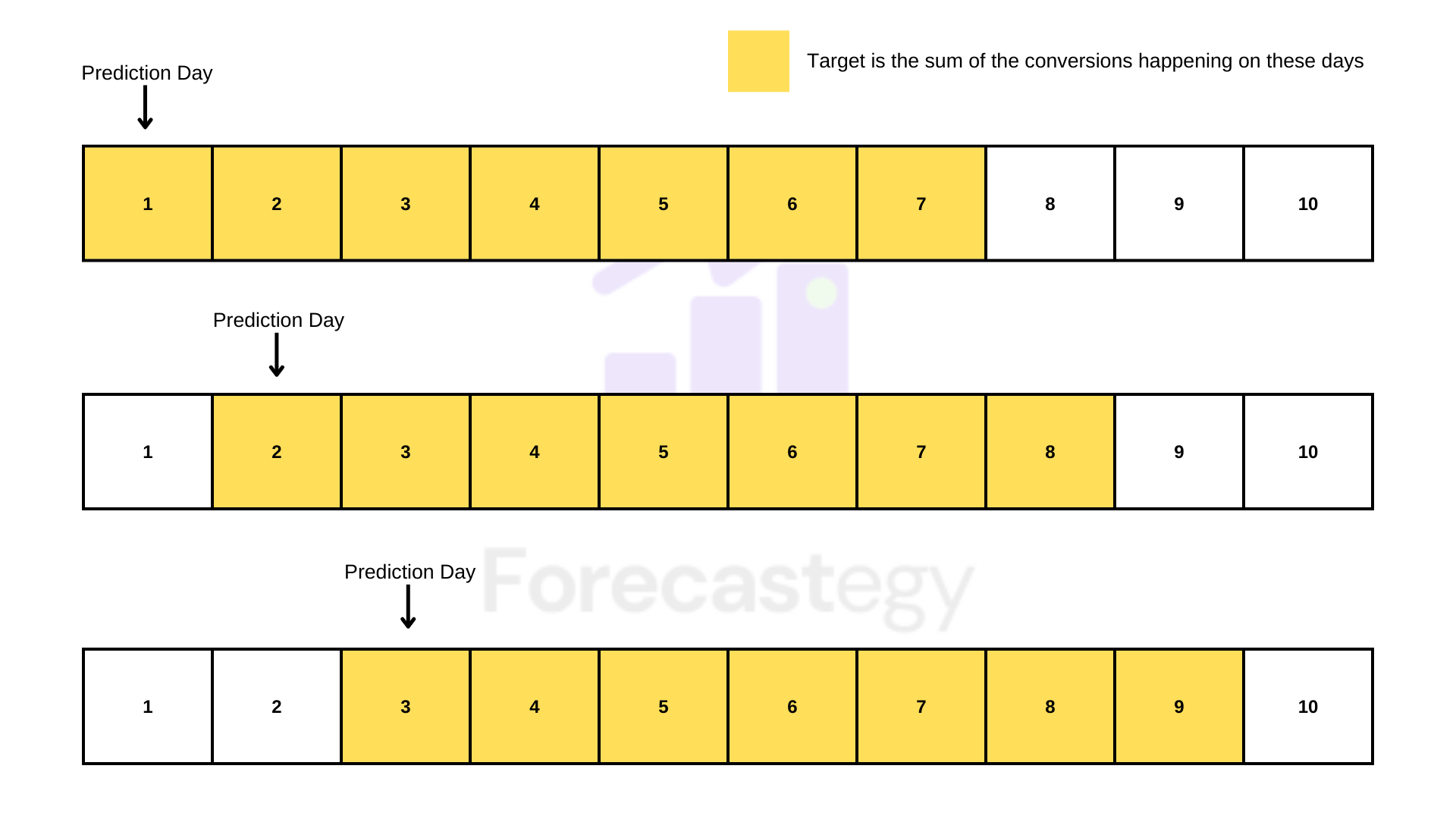
The target becomes the sum of conversions in a fixed number of days. Like in this visual:

Instead of predicting only the next day’s sales, we predict the sum of sales for the next few days.
This allows me to use daily data and still have a lot of non-zero targets. It can even help account for adstock in a forward-looking way.
A crazy thought: even if you have multiple conversions every day, you could try modeling sub-daily granularity (e.g. how many sales in the next 12 hours) and use the model to inform day-to-day campaign management.
Let me explain how I did it and what happened.
The Technical Setup
I created a simplified setup based on my readings about traditional marketing mix models, Robyn and LightweightMMM.
From Robyn, I borrowed the Ridge regression, the geometric decay adstock, and the organic media coefficients.
From LightweightMMM, I borrowed the Bayesian approach, weekday seasonality, and exponential trend. I ended up removing the trend because it wrecked my out-of-sample performance.
I used scikit-learn. By Bayesian I mean using BayesianRidge instead of Ridge.
On the surface, it seems fine to use Robyn or LWMMM with this target transformation, but I wanted to do it in a fully-controlled, familiar environment, to make sure I understood what was going on.
Weekday seasonality was a simple one-hot encoding of the weekday.
The Theta for geometric decay adstock was fixed at 0.95 based on previous knowledge of the data.
The input data columns are paid and organic media channels plus encoded weekday. Units are impressions.
We have 214 days to train, and 91 days to test. Each row/example corresponds to a day of adstocked impressions.
I will talk about “days” instead of steps or periods, but you can generalize it as a discrete time step.
I used a window size of 7 days because it’s what makes sense for my data. The method is valid for other sizes too.
The Y-axis of any plot was scaled by dividing by the max absolute value. Each X-axis period is a week. I don’t want competitors snooping into my naked sales data.
In modeling time series, we need to be careful of using data from the same day as inputs, as this can leak target information.
A rule of thumb I have is asking: “Will I be able to compute this input with the data I will have when I need to make new predictions in production?”
Considering we are not using target lags as inputs, the impressions of the same day influence the results, and we want to use this model to simulate and optimize a budget, it’s fine.
To evaluate, I chose a non-overlapping, sliding window, time-series validation method that accounts for model retraining with fresh data.
Here’s what it looks like:
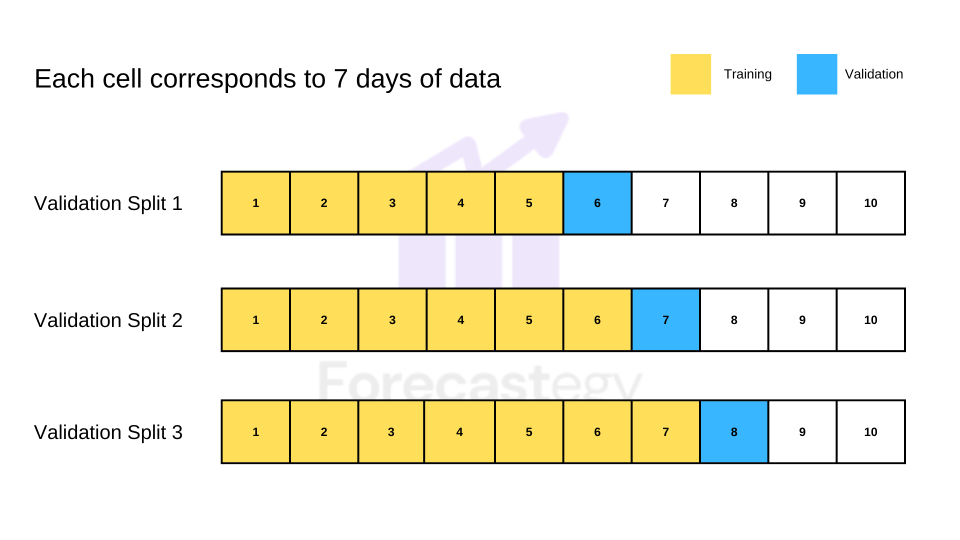
We train the model with data up to that point (expanding) and evaluate it on data from a fixed (sliding) window. I tried dropping old data from training, but it was worse out-of-sample for all the models.
I had to create a gap in the data to avoid leakage on the rolling window model, it’s explained later.
To account for data freshness I used a sample weight that decreases as you go back in time.
Specifically, a sequence of numbers from 1 to N (number of training examples) to the power 0.9. The first data point weight is 1**0.9, last data point weight is N**0.9.
It was inspired by the trend transformation of LightweightMMM.
The Baseline Model
I created the same model, with the same parameters and data, but predicting only one day, to see if the new approach improves over a strong baseline.
It’s very similar to the models I read about, with a few tuning adjustments to make it harder to beat.
It didn’t make sense to compare predictions for each day, but only for a full period. The specific day a conversion happens in a 7-day window is almost random in my data.
So I summed the predictions for the 7 days of the validation period and compared the result to the respective total amount of conversions.
As long as the model can predict how many conversions I will have in the next 7 days, I am happy.
In my experience, summing one-step predictions is not as effective as directly predicting the sum, but you can always find exceptions, so it’s good to try.
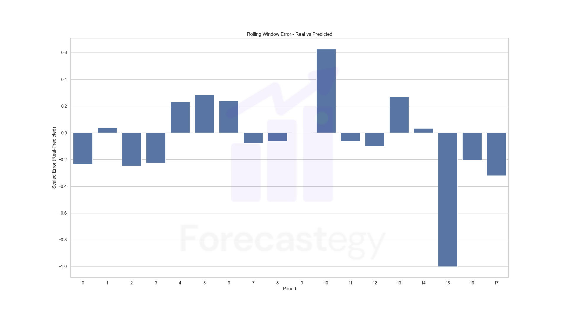
Here are the non-absolute scaled errors by period:
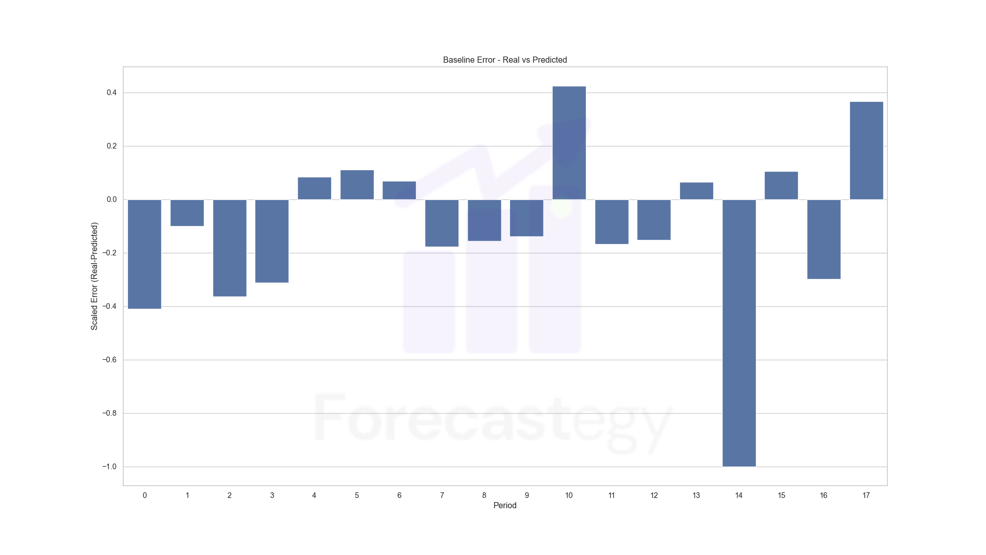
The model is good in general (MAPE: 63.58% and RMSLE: 37.05%) but struggles in the last validation periods. It’s a period I aggressively shifted the budgets, so the model is trying to learn from the new data.
The errors may look high, but we are talking about a small number of conversions, so predicting 3 when it was 2 already inflates it. During modeling I monitored Mean Absolute Error too.
With the baseline set, let’s try the new method!
Predicting The Number Of Conversions In A Rolling Window With A Fixed Size
For each day of data (row), the target was: how many conversions will I have today plus the next 6 days?
I picked “today plus six” days because I usually sell at least one course in any random 7-day period.
To evaluate, I took the prediction on the first day (row) of validation to compare it with the total conversions for the validation period.
Our target is the sum of 7 days, so the prediction of the first day already covers the full period.
Beware Of Leakage!
It’s VERY EASY to leak target information when doing progressive validation with a windowed target if you transform the target before doing the validation split.
Split first and be safer.
Always check every timestamp on the tails of your training and validation data multiple times to make sure you are not making a mistake.
To illustrate:
Let’s say the last example date of my training data is April 7, 2022, and I used April 7 to April 13 to compute the respective target.
Then the first example date on my validation data is April 8, 2022, which I used from April 8 to April 14 to compute the respective target.
It means I just broke my validation by training on a target that covers part of my out-of-sample data.
In this case, I have to delete any training data row after April 1.
In practice, it means introducing a gap between the training and validation data for this model, like this:
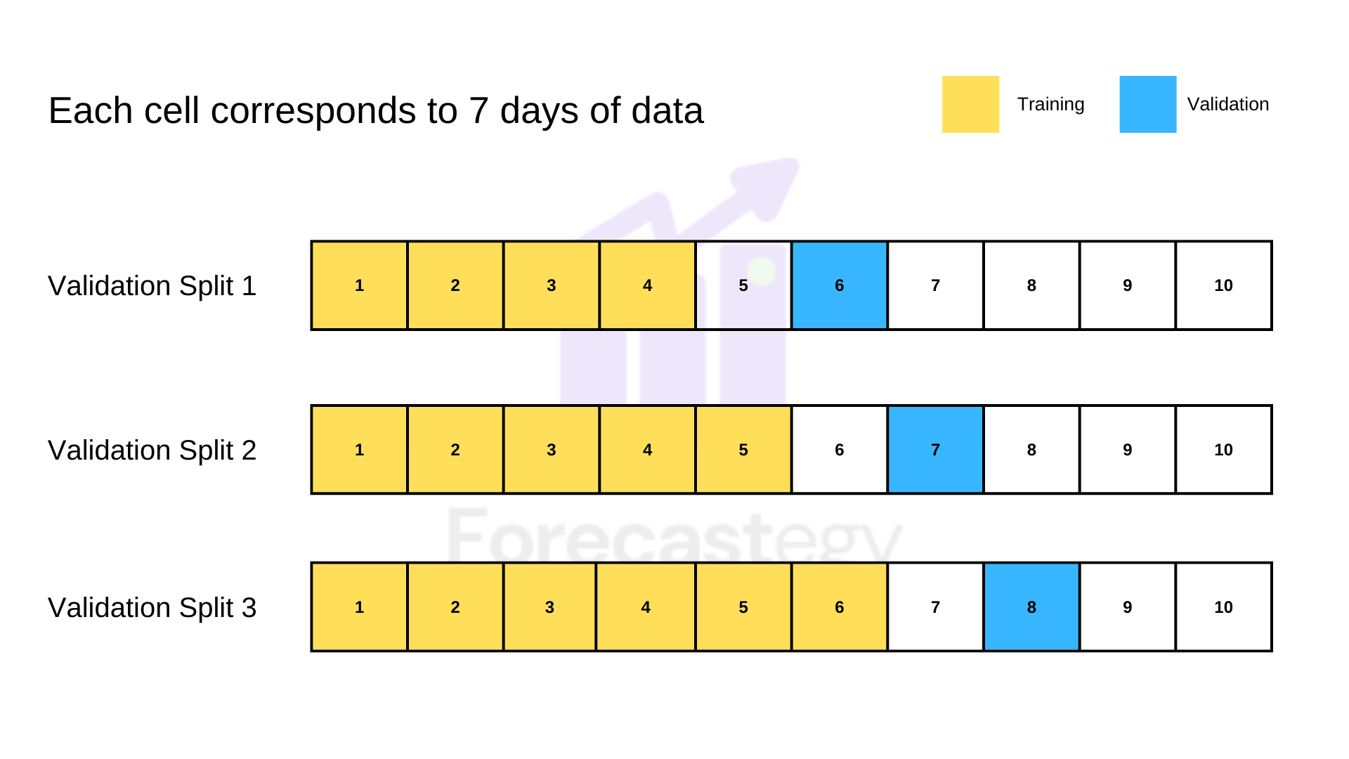
This model beats the baseline with MAPE: 41.01% and RMSLE: 31.33%.
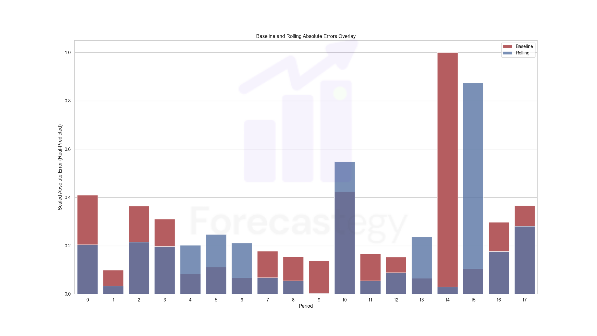
Here is the out-of-sample performance, over the same periods as the baseline model:
This is just to look at the behavior of the model through time.
To have a better idea of how they compare I took the absolute value of the errors and scaled them by the maximum across the two models:
Blue-ish is the rolling window target model. Red is the baseline.
Satisfied with the results, I wanted to see how the performance of the models correlated across periods.
The Spearman correlation of the errors is 0.39. The same for predictions is 0.71.
They are different enough to be good as an ensemble (e.g. a weighted average of their predictions instead of using only one model). Why not try it?
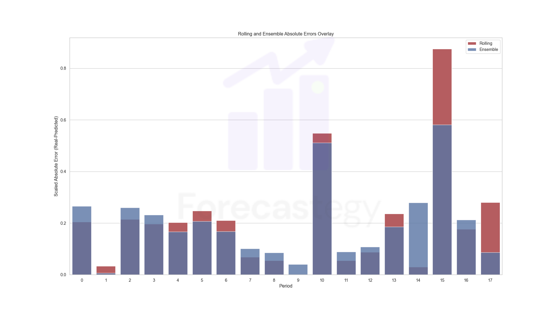
I tried a few combinations that slightly improved RMSLE but not MAPE. There is an additional benefit of making ensembles: the predictions become more stable.
Here is the comparison with the rolling window model. (Blue-ish is the ensemble now)
Final Thoughts
Predicting the sum of multiple days at the same time worked! 🎉
It’s the first time I try to move away from traditional marketing mix modeling and experiment with machine learning ideas to improve it, so I am happy it worked.
This is not a panacea. It’s another tool to keep in the toolbox.
The most important takes are the rolling window target and the progressive time-series validation.
They seem essential to unlock higher granularity in low-conversion environments and can help you go to intraday granularity if you have high-conversion daily data.
Robyn seems to do an internal time-series validation, but I didn’t investigate the code to see their approach.
Out-of-sample metrics are much more valuable than just looking at in-sample statistical tests.
I have seen many models with great in-sample metrics make terrible predictions, but it’s much less common to see models with stable repeated out-of-sample validation metrics do poorly.
Happy modeling! (And please share the article if you liked it, thanks! 🙂)
Here is the link if you want to see my previous marketing mix model on this data