In this tutorial, we’ll explore some practical techniques to measure the similarity between time series data in Python using the most popular distance measures.
To make sure that the results are not affected by noise or irrelevant factors, we’ll apply techniques such as scaling, detrending, and smoothing.
Once the data is preprocessed, we can use simple distance measures like Pearson correlation and Euclidean distance to measure the similarity of two aligned time series.
However, in real-world scenarios, time series may not be aligned, or they may have different lengths.
In such cases, we’ll explore a more advanced technique called Dynamic Time Warping (DTW).
Get ready to dive deep into the world of time series similarity measures and learn some exciting techniques to boost your Python skills.
Let’s get started!
Preprocessing Time Series Data For Similarity Measures In Python
Before we can measure the similarity between two time series, it’s a good idea to preprocess the data to make sure that the results will not be affected by noise or factors that have nothing to do with the similarity.
The three most common preprocessing techniques are scaling, detrending, and smoothing.
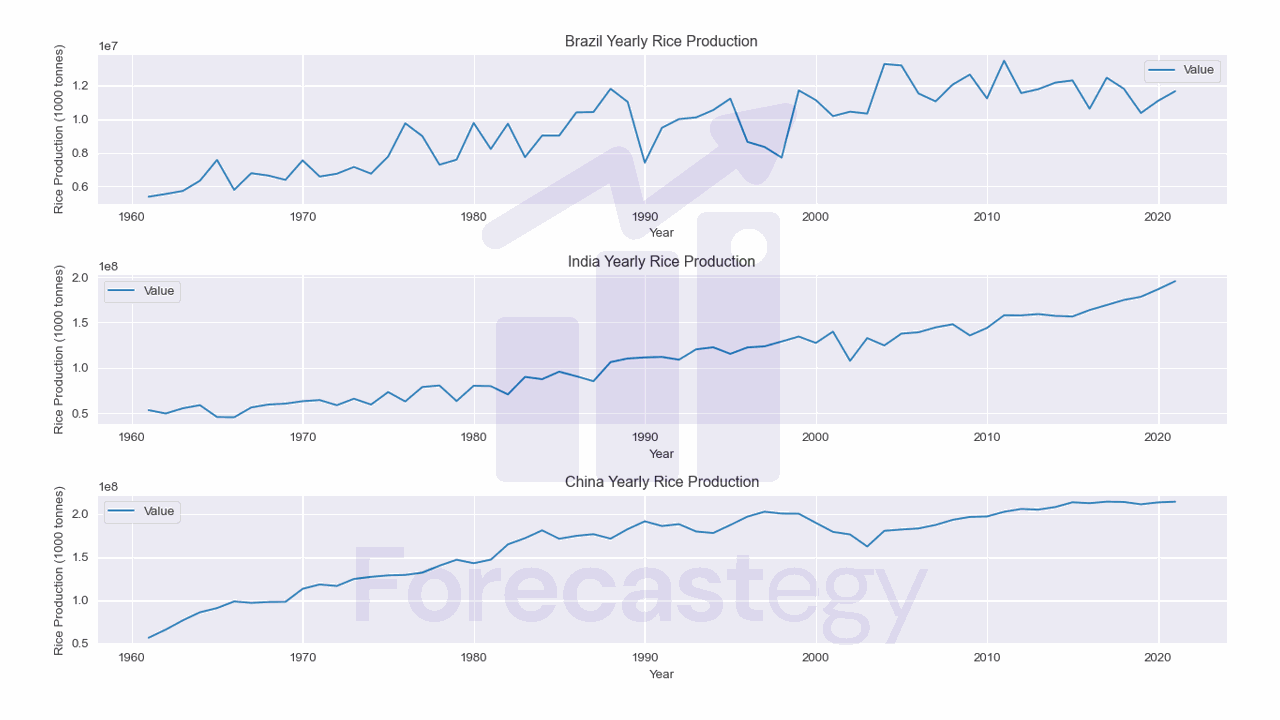
Let’s load data from yearly rice production of Brazil, China, and India to understand how these techniques work.
import pandas as pd
import numpy as np
from matplotlib import pyplot as plt
import os

data = pd.read_csv(os.path.join(path, 'rice production across different countries from 1961 to 2021.csv'))
selected = ['Brazil', 'India', 'China']
data = data.loc[data['Area'].isin(selected)]
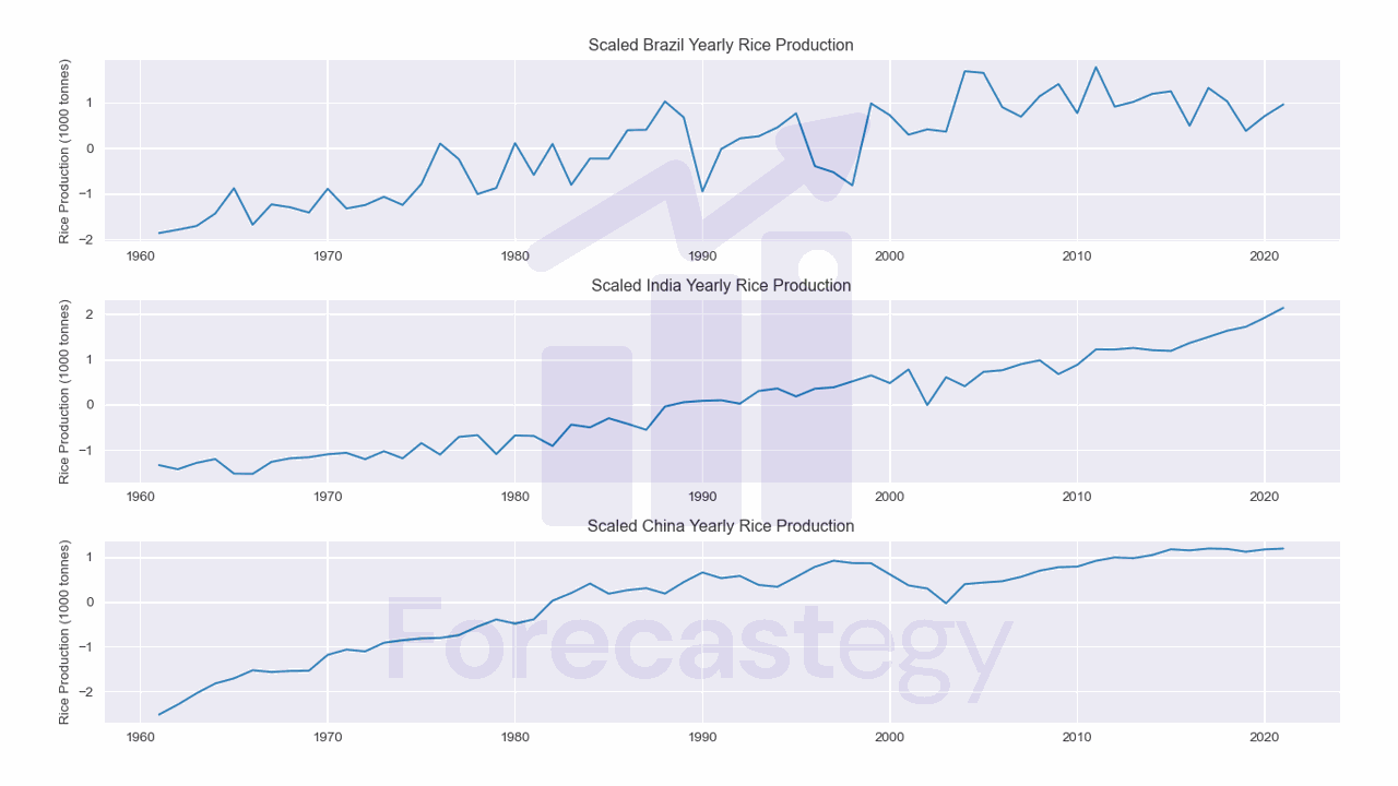
Scaling
Scaling is the process of subtracting the mean of the time series from each value and then dividing the result by the standard deviation of the series.
This is the same transformation that is applied to the data when using the z-score normalization.
You can find it named time series normalization, scaling, or standardization.
scaled = dict()
for area in data['Area'].unique():
    series = data[data['Area']==area]['Value'].values
    scaled[area] = (series - series.mean()) / series.std()
scaled = pd.DataFrame(scaled)
| Brazil | China | India | |
|---|---|---|---|
| 1961 | -1.86774 | -2.50948 | -1.33578 |
| 1962 | -1.79355 | -2.28856 | -1.42553 |
| 1963 | -1.71083 | -2.03712 | -1.28679 |
| 1964 | -1.43779 | -1.81721 | -1.20203 |
| 1965 | -0.880431 | -1.70387 | -1.52196 |
We scaled, but we still have a trend.
Sometimes you want to keep the trend if it’s important for your analysis. In any case, I will show you how to remove it.
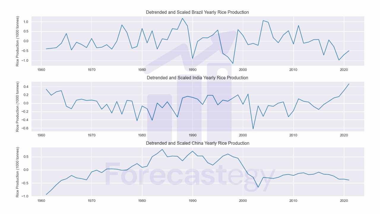
Detrending
Detrending is the process of removing any trend from the time series.
If we want to measure the similarity of the underlying patterns, not the trend, we can perform detrending using scipy.signal.detrend.
from scipy.signal import detrend

detrended = dict()
for area in selected:
    detrended[area] = detrend(scaled[area])
detrended = pd.DataFrame(detrended, index=sorted(data['Year'].unique()))
| Brazil | India | China | |
|---|---|---|---|
| 1961 | -0.403679 | 0.335164 | -0.936089 |
| 1962 | -0.378289 | 0.189715 | -0.767612 |
| 1963 | -0.344379 | 0.272754 | -0.568622 |
| 1964 | -0.12014 | 0.301818 | -0.401155 |
| 1965 | 0.38842 | -0.0738108 | -0.340266 |
This will fit a least-squares model to the data and then subtract it.
Here, scaled is the scaled data from the previous step, and detrended is the detrended data.
You can see the data between Brazil and India seems easier to compare, while China is still a bit different.
Another step we can take is to smooth the data to remove noise that can affect the similarity measures.
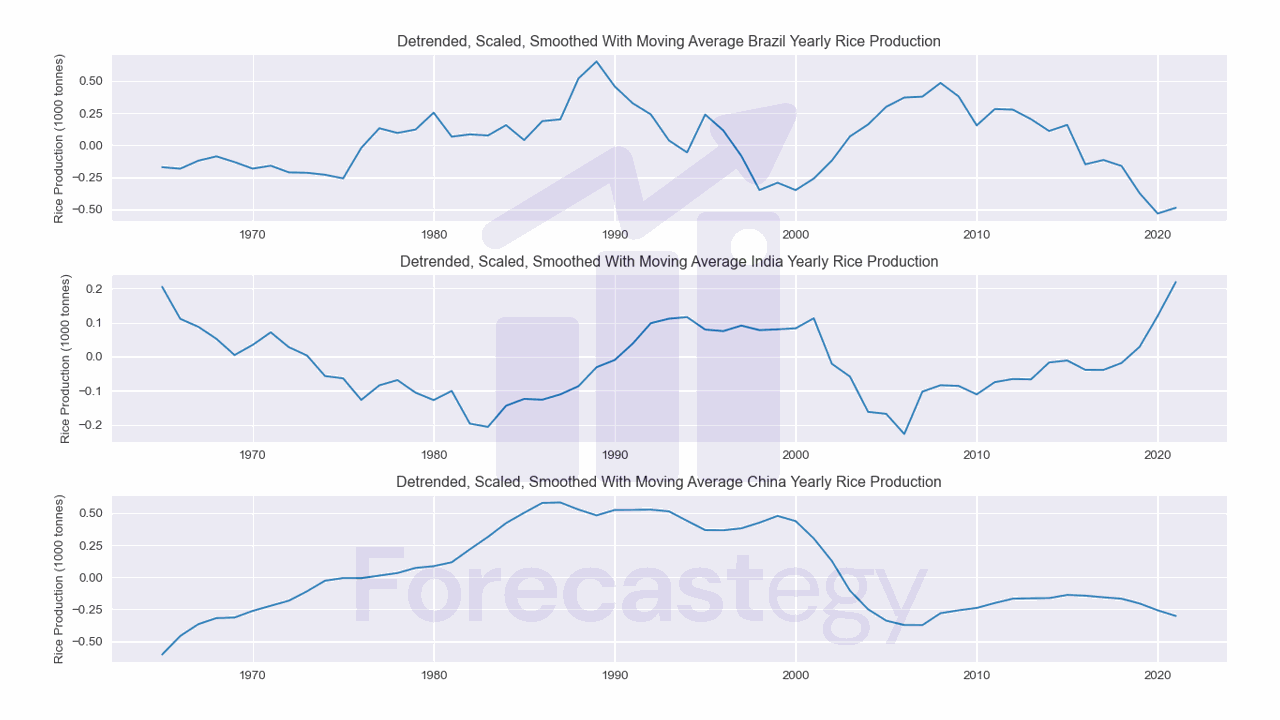
Smoothing
Smoothing is the process of removing noise from the time series.
It can be as simple as taking a moving average of the data.
smoothed = detrended.rolling(5).mean().dropna()
Smoothing with a moving average comes from the assumption that the average of the data is a better representation of the underlying pattern than the individual data points.
This code will calculate a rolling average of the data using a window size of 5. You can try different window sizes to see how it affects the results.
I dropped the first 4 rows because they contain NaN values.
| Brazil | India | China | |
|---|---|---|---|
| 1965 | -0.171613 | 0.205128 | -0.602749 |
| 1966 | -0.18346 | 0.111086 | -0.458108 |
| 1967 | -0.12075 | 0.0876422 | -0.36545 |
| 1968 | -0.0871858 | 0.0522224 | -0.318492 |
| 1969 | -0.131532 | 0.00475607 | -0.314201 |
You can see the data is less “jagged” now.
A fancier way to smooth the data is to use a Savitzky-Golay filter.
from scipy.signal import savgol_filter

savgol = dict()
for area in selected:
    savgol[area] = savgol_filter(detrended[area], window_length=5, polyorder=1)
savgol = pd.DataFrame(savgol, index=sorted(data['Year'].unique()))
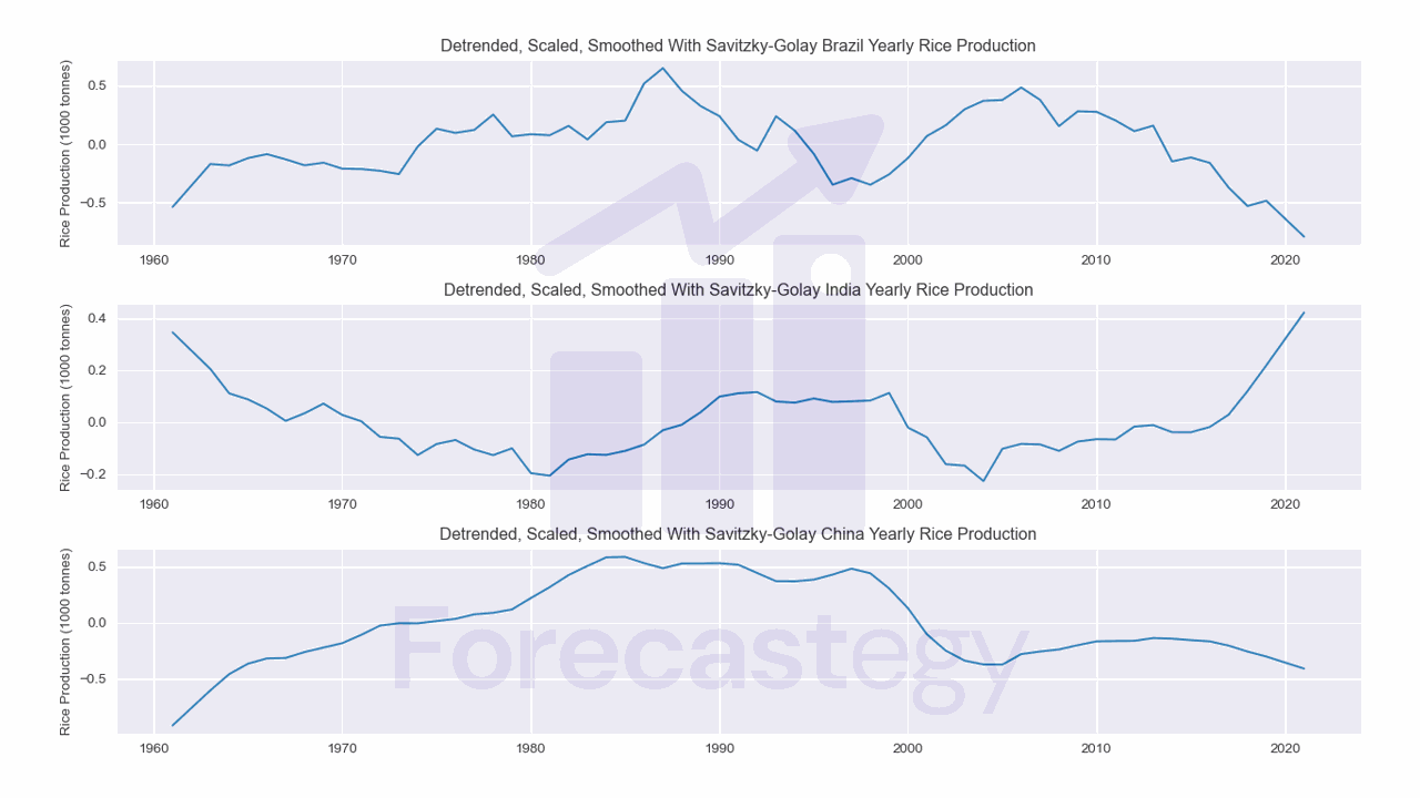
To use this filter, we need to specify the window length and the polynomial order.
The window length is the number of data points used to calculate the filter.
The polynomial order is the order of the polynomial used by the filter to fit the data.
Which Preprocessing Method Is Best?
I like to take the “practical machine learning” approach to this problem.
You don’t need to use all the preprocessing methods I showed you, or even use them in the same order.
Try different preprocessing methods and see which one gives you the best results according to your metrics or experience.
Results that move too far from your expectations are usually wrong or demand a lot more investigation before you can trust them.
Another method you can use is differencing.
Simple Distances For Time Series Similarity
After preprocessing the data, we can use simple distance measures to measure the similarity between two time series.
Pearson Correlation
Pearson correlation is a measure of the linear correlation between two time series.
It was used as an official metric by two financial forecasting competitions on Kaggle: the G-Research Crypto Forecasting and the Ubiquant Market Prediction.
We can calculate the Pearson correlation coefficient directly in pandas with df.corr.
smoothed.corr()
| Brazil | India | China | |
|---|---|---|---|
| Brazil | 1 | -0.554765 | 0.205345 |
| India | -0.554765 | 1 | -0.00622666 |
| China | 0.205345 | -0.00622666 | 1 |
This function gives us the correlation between all pairs of time series in an organized table, which is very convenient.
Pearson correlation varies between -1 and 1. -1 means the time series are perfectly negatively correlated (one goes up when the other goes down), 1 means the time series are perfectly positively correlated (one goes up when the other goes up), and 0 means the time series are not correlated at all.
Anything in between means they are correlated (the direction depends on the signal), but not perfectly.
For example, the correlation between Brazil and India is -0.55, which means that rice production in Brazil tends to go down when rice production in India goes up and vice versa.
But be careful! This is not a measure of causation. It only means that this is what happened in the historical data.
Euclidean Distance
The Euclidean distance is a widely used technique to measure the similarity between time series.
It is a simple and intuitive measure that calculates the distance between two time series as the straight-line distance between their corresponding points.
We can easily calculate it with the euclidean_distances function from scikit-learn.
from sklearn.metrics.pairwise import euclidean_distances

euc_dist = euclidean_distances(smoothed.T)
pd.DataFrame(euc_dist, index=selected, columns=selected)
| Brazil | India | China | |
|---|---|---|---|
| Brazil | 0 | 2.50487 | 2.8451 |
| India | 2.50487 | 0 | 2.66397 |
| China | 2.8451 | 2.66397 | 0 |
Notice that we pass the transpose of the dataframe to the function. This is because the function expects the time series to be in the rows, not the columns.
And remember we are calculating a distance, not a similarity. The smaller the distance, the more similar the time series are.
One of the benefits of using the Euclidean distance is its simplicity and ease of implementation. It is a straightforward measure that requires minimal computation, making it a suitable choice for large datasets.
However, it has some drawbacks. The Euclidean distance is sensitive to outliers and it is not scale-invariant. This means that the distance between two time series will be different depending on the scale of the data.
In our example, the data is already scaled, so this is not a problem.
Dynamic Time Warping
Dynamic Time Warping (DTW) is a more advanced technique for measuring the similarity of time series.
DTW can handle time series that are not aligned and also series with different lengths, which happens a lot in real-world data.
In this dataset, some countries have been producing rice for a long time, and others have only started recently, although our selected countries have full data.
DTW works by warping the time axis of one time series to match the time axis of the other time series.
This technique was very successful in the Driver Telematics Analysis competition, where the goal was to identify drivers by looking at their driving behavior.
The main drawback of DTW is that it is computationally expensive. It can take a long time to calculate the distance between two time series, which can be a problem if you have many comparisons to make.
Anyway, the DTAIDistance library implemented a fast version of DTW in C that we can use in Python.
from dtaidistance import dtw

dtw_dist = dtw.distance_matrix_fast(smoothed.T.values)
pd.DataFrame(dtw_dist, index=selected, columns=selected)
| Brazil | India | China | |
|---|---|---|---|
| Brazil | 0 | 1.74072 | 1.44652 |
| India | 1.74072 | 0 | 2.17045 |
| China | 1.44652 | 2.17045 | 0 |
Notice that we need to transpose the dataframe, because the function expects the time series to be in the rows instead of the columns, and we need to convert it to a numpy array with the .values attribute.
Here, the smaller the distance, the more similar the time series are.
If you compare the results of the Euclidean distance and the DTW, you will notice that they are different.
Keep this in mind when you are choosing a distance measure. Each can give you different results.
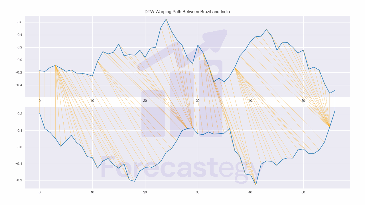
We can plot the warping path between two time series with the plot_warping function.
from dtaidistance import dtw_visualisation as dtwvis

fig, ax = plt.subplots(2,1,figsize=(1280/96, 720/96))
path = dtw.warping_path(smoothed['Brazil'].values, smoothed['India'].values)
dtwvis.plot_warping(smoothed['Brazil'].values, smoothed['India'].values, path,
                    fig=fig, axs=ax)
ax[0].set_title('DTW Warping Path Between Brazil and India')
fig.tight_layout()

This shows us which points in one time series are best aligned with which points in the other time series.
It can be useful to identify shifted patterns in the time series.