There’s a very interesting marketing mix modeling approach published by Uber’s data science team that uses coefficients that vary over time to estimate a media channel’s effects.
The modeling approach is called Bayesian Time-Varying Coefficients (BTVC) and it’s available on Orbit, their forecasting package, as Kernel Time-Varying Regression.
Instead of getting a single coefficient to understand each media effect, we can see how the effect varied through time with confidence intervals.
It’s another tool to have in your toolbox when you need to create a marketing mix model or do any time series modeling.
More than that, we can fit multiple models, like LightweightMMM, Robyn, and BTVC, and combine their results to get more stable estimates of the true media effects.
Here I will show how I followed Uber’s paper to build a marketing mix model using BTVC.
Getting Advertising Data
We are going to use the same dataset from LightweightMMM’s tutorial
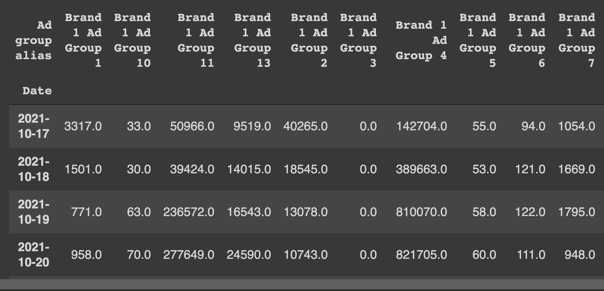
Here we have data from ad campaigns that ran on multiple marketplaces and the sales that likely resulted from them.
We will use Impressions as the features and Sales as the target.
Both date and the target need to be in the same DataFrame for Orbit. We will pass the names of these columns to the model object later.
data = pd.read_excel("/content/Sr Advertising Analyst Work Sample (1).xlsx")

agg_data = data.groupby(["Date", "Ad group alias"])[["Impressions","Spend", "Sales",]].sum()
agg_data = agg_data.drop(["Brand 1 Ad Group 12"], axis=0, level=1) # zero cost train


media_data_raw = agg_data['Impressions'].unstack().fillna(0)
costs_raw = agg_data['Spend'].unstack()
sales_raw = agg_data['Sales'].reset_index().groupby("Date").sum()
media_data_raw["Sales"] = sales_raw

media_data_raw = media_data_raw.reset_index()
I tried scaling the data with scikit-learn’s StandardScaler and MaxAbsScaler. MaxAbsScaler worked better, I guess because of the zeros in the data, but I didn’t investigate further.
MaxAbsScaler simply divides each column value by the maximal absolute value it can find on the column.
Target was scaled using a separate MaxAbsScaler.
date_col = "Date"
response_col = "Sales"

regressor_col = ['Brand 1 Ad Group 1', 'Brand 1 Ad Group 10',
       'Brand 1 Ad Group 11', 'Brand 1 Ad Group 13', 'Brand 1 Ad Group 2',
       'Brand 1 Ad Group 3', 'Brand 1 Ad Group 4', 'Brand 1 Ad Group 5',
       'Brand 1 Ad Group 6', 'Brand 1 Ad Group 7', 'Brand 1 Ad Group 8',
       'Brand 1 Ad Group 9', 'Brand 2 Ad Group 1', 'Brand 2 Ad Group 2',
       'Brand 2 Ad Group 3', 'Brand 2 Ad Group 4', 'Brand 2 Ad Group 5',
       'Brand 1 Ad Group 14', 'Brand 2 Ad Group 6']
split_point = -28 # 28 days to end of data

media_data_train = media_data_raw.iloc[:split_point].copy()
media_data_test = media_data_raw.iloc[split_point:].copy()

scaler = MaxAbsScaler() # better than standard
media_data_train.loc[:, regressor_col] = scaler.fit_transform(media_data_train.loc[:, regressor_col])
media_data_test.loc[:, regressor_col] = scaler.transform(media_data_test.loc[:, regressor_col])

scaler_y = MaxAbsScaler()
media_data_train.loc[:, response_col] = scaler_y.fit_transform(media_data_train.loc[:, response_col].values.reshape(-1,1))

media_names = media_data_raw.columns
I consider the scaling method as a hyperparameter, so try a few in your data before committing.
The validation was a simple time split, with the last 28 days as the validation set, like in the other tutorial.
Building the Model
We need to pass a list of columns to use as regressors (inputs).
If we don’t, Orbit will only create a simple time series model with the target variable and date, which is not our goal here.
We can specify seasonality. Here I put 7 to allow for weekday seasonality, but if we had more data, we could put 365.25 as they suggest in the documentation, to capture yearly seasonality effects (like Christmas and Black Friday).
import orbit
from orbit.models import KTR

ktr_ = KTR(
    response_col=response_col,
    date_col=date_col,
    regressor_col=regressor_col,
    #regressor_sign=["+"]*len(regressor_col), # strictly positive signs hurt MAPE but can be useful to interpret?
    seed=2021,
    seasonality=[7], # cant use 365 seasonality because have only 59 rows
    estimator='pyro-svi',
    n_bootstrap_draws=1e4,
    num_steps=301,
    message=100)

ktr_.fit(media_data_train)

predicted_df = ktr_.predict(df=media_data_test)
There are a few hyperparameters you can tune like the learning rate of the SVI estimator and the number of steps (iterations) the model will take.
The default values from the documentation worked very well for this data, achieving the same error as LightweightMMM.
Always be careful when tuning models with a small amount of data, like it’s usually the case when doing marketing mix models, but don’t be afraid to play a little.
After checking the out-of-sample error, I retrained the model with all the data.
Estimating Media Effects
There are two big applications I see for marketing mix models: understanding ROI/media effects and optimizing advertising budgets.
Thinking like an ad buyer, the first seems much more important, while the second is better taken as a suggestion of where I should put my advertising dollars.
One very cool feature of Orbit is to plot the regression coefficients over time.
ktr_.plot_regression_coefs(figsize=(10, 30), include_ci=True)
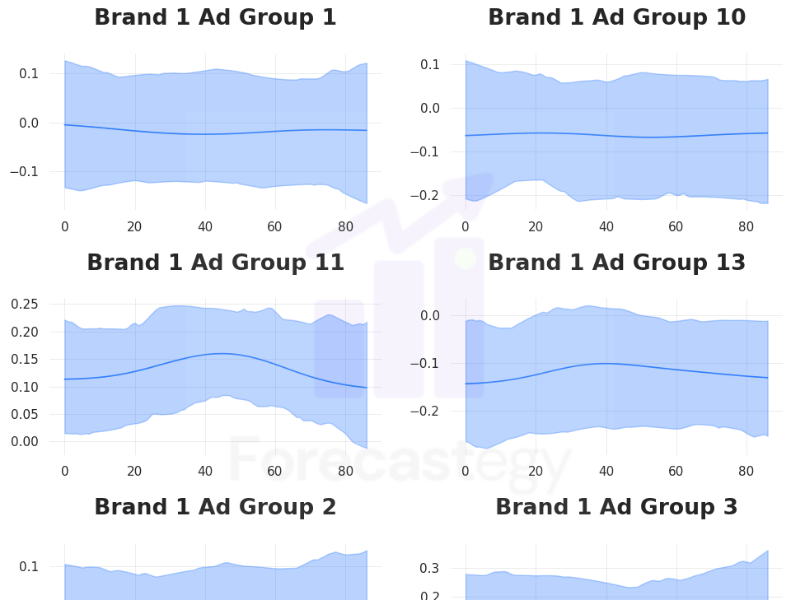
This not only shows the estimated media effect of the channels today but shows how they may have influenced sales through time.
Why is this useful?
Social media campaigns tend to saturate very fast.
Depending on the budget, you have to “refresh creatives” weekly, which means launching new ads and ad sets because the current ones have been shown multiple times to the people you want.
This can be captured by the changes in coefficients over time and help you understand the types of ads and audiences that tend to have a longer lifetime.
Another way to use it is to understand how different is the lifecycle of a campaign in different ad networks like Tiktok, Facebook, and Google.
I would guess the coefficients from a Google campaign will be much more stable than a Tiktok one.
Negative Coefficients
I didn’t constrain the coefficients to be positive, so we got negative coefficients which can be hard to interpret.
Orbit has the capability to force positive-only coefficients, but the out-of-sample error more than doubled.
There is probably a way to fix this by changing priors and hyperparameters, but I still didn’t find how to do it.
I am not sure how big of a problem this is in practice.
Negative coefficients may arise because of problems during the model estimation, but if they are real, they can tell us useful information.
Estimating Return on Investment (ROI)
Unfortunately, we don’t have ROI estimation for the channels, as this is not a specialized marketing mix library, but we can use the media effects to calculate it.
So I decided to calculate it manually.
DISCLAIMER: The following code/calculations part has a high risk of having mistakes as it’s the first time I attempt to calculate contribution and ROI from scratch. So take everything with a grain of salt.
I loosely followed the instructions shared in this tutorial.
The basic idea is to multiply the coefficients for each media channel by the number of impressions to get the estimation of that specific channel.
As we have contributions for each time step, we sum up everything and find each media channel’s contribution.
contribution = scaler_y.inverse_transform(ktr_.get_regression_coefs().iloc[:, 1:] * media_data_full[regressor_col])
contribution = pd.DataFrame(contribution,columns=regressor_col).sum(axis=0)
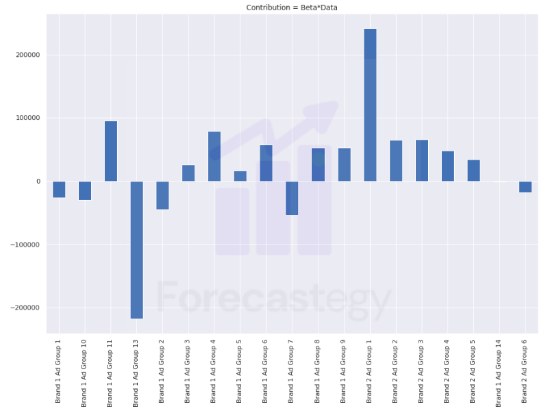
Most of the contributions are positive, which I guess is good.
To get the ROI we simply divide the unscaled contribution by the total money spent on that channel.
roi = (contribution.sum(axis=0) / costs_raw.sum(axis=0)).clip(0)
I clipped the negative values to zero to make it easier to visualize.
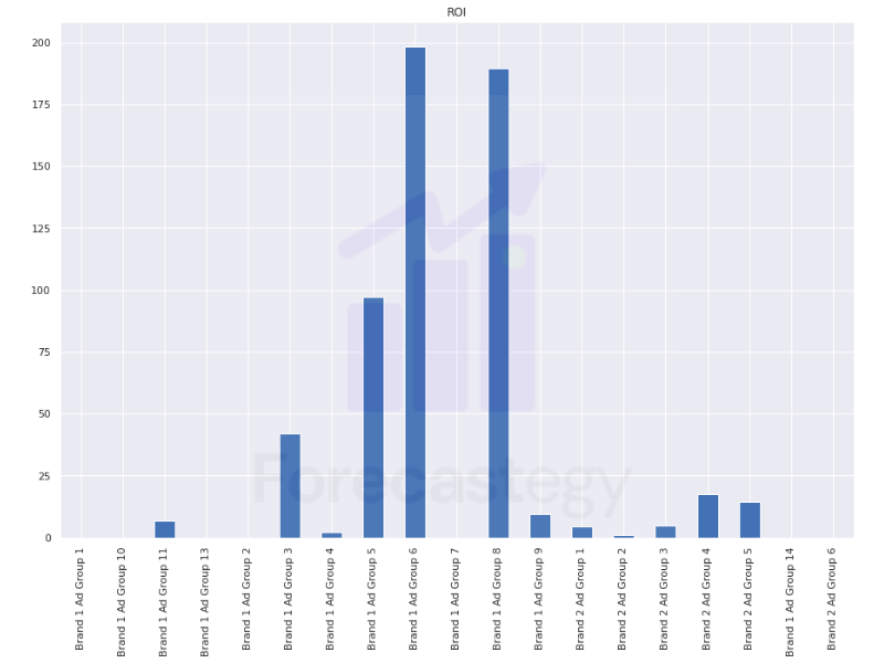
I guess we should think of these numbers more as directional guides than taking them as precise estimates of true ROI.
Some of them look very inflated, but they might be very targeted remarketing campaigns for repeated customers which would have astounding returns on a very small budget.
Always remember to validate your marketing mix modeling finds with experiments!
Optimizing Advertising Budgets
Just like we don’t have a native ROI function, we don’t have a budget allocation optimizer on Orbit.
So I used this opportunity to play with Nevergrad, a gradient-free optimization library that powers Robyn.
The same disclaimer is valid here. This code is just a quick and dirty first draft of a possible optimizer.
My goal is to get the optimal impressions I should have in each ad group, taking into account the cost per impression for that ad group.
The cost per impression is always rising, but we can use our training data costs to have a good estimate for the near future.
Now we need an optimization function that takes a suggested allocation and returns the ROI.
I wrote this function takes the allocation suggested by the Nevergrad optimizer, scales it, puts it in the format that Orbit likes, generates the predicted revenue, and divides it by the estimated cost.
There is still the problem of an unlimited budget.
As it was the first time I used Nevergrad, I still didn’t understand how to constrain the total cost during the optimization, so I just set the function to return 1 when the cost of the allocation goes over a specified number (2,000 here).
cpi = costs_raw.sum(axis=0) / media_data_raw.sum(axis=0)
cpi = cpi[regressor_col]

def opt_fun(*x):
  x = np.array(x).reshape(1,-1)

  x_ = media_data_full.iloc[-1:].copy()
  x_['Date'] = x_['Date'] + pd.Timedelta(1, "D")

  x = pd.DataFrame(x, columns=regressor_col)
  cost = (cpi * x).squeeze().sum() # unlimited budget
  if cost > 2000:
    return 1

  x__ = scaler.transform(x)
  x_[regressor_col] = x__

  p = scaler_y.inverse_transform(ktr_.predict(x_)['prediction'].values.reshape(-1,1))[0][0]
  return -(p / cost)
As we will use the minimize function, we optimize for “negative ROI”.
Following an idea from LightweightMMM, I set the upper bound of each ad group (media channel) as 1.1 times the maximum impressions we have seen in the training data.
Channels are not infinitely scalable, so I am assuming we can just go 10% above the maximum we ever saw.
import nevergrad as ng

params = ng.p.Instrumentation(*[ng.p.Scalar(lower=0, upper=b*1.1) for b in media_data_raw.max(axis=0).iloc[1:-1].values])
optimizer = ng.optimizers.RandomSearch(parametrization=params, budget=100)
recommendation = optimizer.minimize(opt_fun)
print(recommendation.value)
The optimal x or recommendation.value is the number of impressions we should buy for each channel.
I am not a big fan of using an optimizer to blindly allocate budgets but it can be a suggestion inside the ad buyer dashboard.
Where Is Adstock?
I was surprised to see the model work well even without applying an adstock transformation to the inputs.
Adstock modeling is a way to compute the lingering effects that seeing an ad will have in the conversion decision of the user.
The paper doesn’t give many details of the specific data processing steps they did for the marketing data, but talk about using adstock as a hyperparameter in their final pipeline.
This data seems to come from marketplace ads, which are at the very end of the customer journey, so I would expect the effects of impressions to be close to immediate.
The above plus the time-varying nature of the coefficients might be why the model worked well without adstock transformations.
Conclusion
This is a first draft of another approach you can try when building a marketing mix model.
I like the Bayesian nature and the time-varying coefficients of BTVC, but at the end of the day, we need to try multiple tools and see which are the most useful for our dataset and use case.
Happy modeling!