In this article, you will learn how to use Orbit, a Python library for Bayesian time series forecasting.
Orbit is a very straightforward library developed at Uber that offers an interface to train Bayesian exponential smoothing models implemented via the probabilistic programming languages Stan and Pyro.
This is a practical guide: the goal here is not to go into the math behind the models, but rather to show how you can use Orbit in practice to forecast time series data using Bayesian models.
Let’s begin by getting an overview of the models available in Orbit.
Installing Orbit
If you are using Windows, I highly recommend you use Windows Subsystem for Linux to run Orbit.
I spent countless hours trying to get PyStan and Pyro (the backends) to work on Windows without success. With WSL, everything runs smoothly.
You can install Orbit with pip.
pip install orbit-ml
Or with conda.
conda install -c conda-forge orbit-ml
Loading the Data For Orbit
We will use real sales data made available by Favorita, a large Ecuadorian grocery chain.
We have sales data from 2013 to 2017 for multiple stores and product categories.
import pandas as pd
import numpy as np
import os

def wmape(y_true, y_pred):
    return np.abs(y_true - y_pred).sum() / np.abs(y_true).sum()

path = 'train.csv'
data = pd.read_csv(path, index_col='id', parse_dates=['date'])

data2 = data.loc[((data['store_nbr'] == 1) & (data['family'] == 'MEATS')), ['date', 'sales', 'onpromotion']]
Orbit can process only a single time series at a time, so I selected one product category (family) and one store to make things easier.
The columns are:
date: the date of the recordsales: the number of items soldonpromotion: the number of products from that category that were on promotion on that day
I created a custom function to calculate WMAPE, which is an adaptation of the mean absolute percentage error that solves the problem of dividing by zero.
The weight of each sample is given by the magnitude of the real value.
This data doesn’t contain a record for December 25, so I just copied the sales from December 18 to December 25 to keep the weekly pattern.
dec25 = list()
for year in range(2013,2017):
    dec18 = data2.loc[(data2['date'] == f'{year}-12-18')]
    dec25 += [{'date': pd.Timestamp(f'{year}-12-25'), 'sales': dec18['sales'].values[0], 'onpromotion': dec18['onpromotion'].values[0]}]
data2 = pd.concat([data2, pd.DataFrame(dec25)], ignore_index=True).sort_values('date')
To validate our models, we will use a simple time split, taking the first 3 months of 2017 as validation data and everything before that as training data.
train = data2.loc[data2['date'] < '2017-01-01']
valid = data2.loc[(data2['date'] >= '2017-01-01') & (data2['date'] < '2017-04-01')]
We will have an internal validation process too, but this comes later.
Orbit’s Bayesian Time Series Forecasting Models
The main difference you will find in Bayesian approaches is that they use priors to estimate the parameters of the model.
So we set up a prior distribution for each parameter, which can be based on our knowledge of the problem or on the data itself.
Then we use the data to update the priors and get a posterior distribution for each parameter.
The posterior distribution is then used to make predictions.
Note: I didn’t include the Local Global Trend (LGT) model in this article because it will be deprecated due to problems with convergence in regression.
Exponential Smoothing (ETS)
Unlike traditional models, Bayesian ETS models make use of prior knowledge in order to update their beliefs as new data becomes available.
This hopefully helps improve the accuracy of predictions and can also help to account for uncertainty in the data, as we get probabilistic forecasts instead of point estimates.
In Orbit’s implementation of ETS the forecasts are a sum of a seasonal and a trend component.
import orbit
from orbit.models import ETS

ets = ETS(date_col='date',
          response_col='sales',
          seasonality=7,
          prediction_percentiles=[5, 95],
          seed=1)
We import ETS from orbit.models and instantiate it with the following parameters:
date_col: the name of the column containing the dateresponse_col: the name of the column containing the response (target) variableseasonality: the number of periods for the model to consider as a season (I put 7 because I want it to consider seasonality for each day of the week)prediction_percentiles: the uncertainty bands we want to computeseed: the random seed. If you get errors saying something about less than zero coefficients, try changing the seed.
We can then fit the model to the training data.
train_ets = train[['date', 'sales']].copy()

ets.fit(df=train_ets)
ETS doesn’t take external regressors, so I created a copy of the training data without the onpromotion column to avoid errors.
For the validation data, we can pass our valid dataframe or generate a new DataFrame with the dates we want to forecast.
I picked the latter because I got many questions about this in other tutorials, so this is how you can do it.
forecast_df = pd.DataFrame({"date": pd.date_range(start='2017-01-01', end='2017-03-31', freq='D')})
p = ets.predict(df=forecast_df)
p = p.merge(valid, on='date', how='left')

print(wmape(p['sales'], p['prediction']))
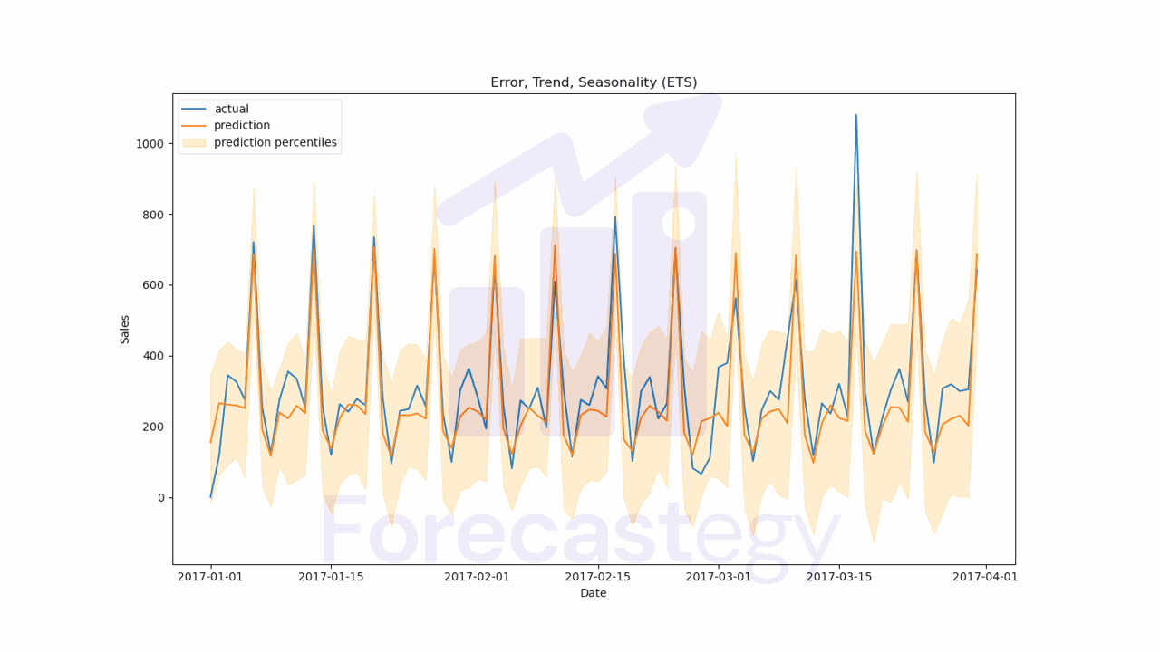
The WMAPE for this model is 21.36%.
I merged the predictions with the validation data to make it easier to compute the WMAPE and plot the results.
fig, ax = plt.subplots(1,1, figsize=(1280/96, 720/96))
ax.plot(p['date'], p['sales'], label='actual')
ax.plot(p['date'], p['prediction'], label='prediction')
ax.fill_between(p['date'], p['prediction_5'], p['prediction_95'], alpha=0.2, color='orange', label='prediction percentiles')
ax.set_title('Error, Trend, Seasonality (ETS)')
ax.set_ylabel('Sales')
ax.set_xlabel('Date')
ax.legend()
plt.show()
It’s very important to visually inspect the results to make sure the model is working as expected.
We can see how well the model forecasts the series with the prediction intervals.

Damped Local Trend (DLT) Model
According to Forecasting: Principles and Practice, constant trend models will overestimate our forecasts as time goes on.
To make the models more stable across longer horizons, we can add a damping factor to the trend component.
This means the trend component will be multiplied by a factor between 0 and 1, which will slowly make the trend go flat in long-term forecasts.
This model takes into account seasonality and can receive external regressors, which are very useful to account for factors beyond the original time series.
The documentation suggests that we use a log-transformed response variable to get better results.
I will show you how to try both options.
DLT gets a few additional parameters:
regressor_col: the name of the columns of the additional featuresregressor_sign: the constraint for the coefficients of the additional features.=means they can be positive or negative,+means they must be positive, and-means they must be negative. This is useful in cases like marketing mix modeling where negative coefficients make no sense.regression_penalty: this is the regularization penalty for the regression. You can consider it a hyperparameter and try any offixed_ridge,auto_ridgeandlasso.damped_factor: this is the factor that will multiply the trend component like explained above. By default it’s 0.8, so I kept this value. You can treat is as another hyperparameter.global_trend_option: the trend takes a deterministic component that can belinear,loglinear,flatorlogistic. I will try all of them to show how you can tune the model.
We will use the BackTester class to create an internal rolling validation process to do the hyperparameter tuning.
from orbit.models import DLT
from orbit.diagnostics.backtest import BackTester

scores = dict()
for global_trend_option in ['linear', 'loglinear', 'flat', 'logistic']:
    dlt = DLT(date_col='date',
            response_col='sales',
            seasonality=7,
            prediction_percentiles=[5, 95],
            regressor_col=['onpromotion'],
            regressor_sign=['='],
            regression_penalty='auto_ridge',
            damped_factor=0.8,
            seed=2, # if you get errors due to less than zero values, try a different seed
            global_trend_option=global_trend_option,
            verbose=False)

    bt = BackTester(df=train,
                    model=dlt,
                    forecast_len=90,
                    n_splits=5,
                    window_type='rolling')

    bt.fit_predict()
    predicted_df = bt.get_predicted_df()

    scores[global_trend_option] = wmape(predicted_df['actual'], predicted_df['prediction'])
We instantiate the model with the same parameters as before, but we change the global_trend_option to try all the options.
We then instantiate the BackTester class with the following parameters:
df: the training datamodel: the model we want to testforecast_len: the number of periods we want to forecastn_splits: the number of splits for the internal validationwindow_type: the type of window we want to use.rollingmeans the validation will be done in a sliding window fashion, whileexpandingmeans the training will be expanded at each split to include all the data up to that point.
I prefer to use rolling because it’s more realistic considering too old data can become irrelevant.
When we call bt.fit_predict(), the BackTester will split the data and run the model for each split.
At the end we can get the predictions with bt.get_predicted_df() and compute the WMAPE.
This is what predicted_df looks like:
| date | actual | prediction_5 | prediction | prediction_95 | training_data | split_key | |
|---|---|---|---|---|---|---|---|
| 0 | 2013-01-01 00:00:00 | 0 | -109.718 | 3.5971 | 110.418 | True | 0 |
| 1 | 2013-01-02 00:00:00 | 369.101 | -116.959 | 9.1862 | 113.618 | True | 0 |
| 2 | 2013-01-03 00:00:00 | 272.319 | -58.2317 | 33.6628 | 137.294 | True | 0 |
| 3 | 2013-01-04 00:00:00 | 454.172 | -67.496 | 31.4584 | 158.862 | True | 0 |
| 4 | 2013-01-05 00:00:00 | 328.94 | -72.577 | 55.4463 | 206.572 | True | 0 |
After computing the WMAPE, we store its value in the scores dictionary for each option.
These were my results:
{'linear': 0.1837287968137849,
 'loglinear': 0.18331473482027125,
 'flat': 0.18415094445622832,
 'logistic': 0.18729231182793238}
The best option on the internal validation was loglinear, so I will use this option for the final model.
best_global_trend_option = min(scores, key=scores.get)

dlt = DLT(date_col='date',
        response_col='sales',
        seasonality=7,
        prediction_percentiles=[5, 95],
        regressor_col=['onpromotion'],
        regressor_sign=['='],
        regression_penalty='auto_ridge',
        damped_factor=0.8,
        seed=2, # if you get errors due to less than zero values, try a different seed
        global_trend_option=best_global_trend_option,
        verbose=False)

dlt.fit(df=train)
Fitting the DLT model is very straightforward, just like the ETS model, it’s inspired by scikit-learn.
This time I decided to pass valid to the predict method because we have the additional information of the onpromotion variable.
In practice, this is a variable we could plan in advance, so we can use it to improve our forecast.
If you have external variables like temperature or a commodity price, you must use an estimate of the future values, even during model development.
Using historical real values when developing the model is a form of data leakage that many people do without realizing. Don’t be one of them.
p = dlt.predict(df=valid[['date', 'onpromotion']])
p = p.merge(valid, on='date', how='left')

print(wmape(p['sales'], p['prediction']))
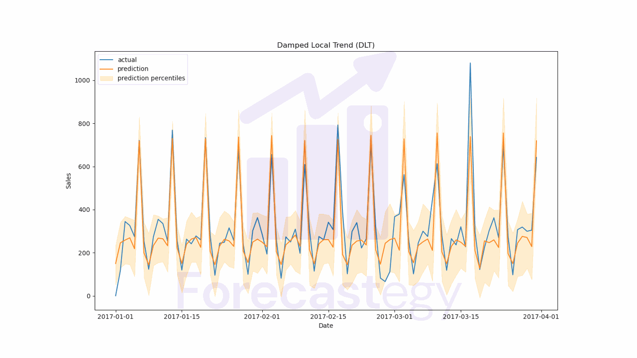
The final WMAPE on the validation set was 20.21%, which is an improvement over the 21.36% we got with ETS. Nice!
This is what the forecast looks like:
fig, ax = plt.subplots(1,1, figsize=(1280/96, 720/96))
ax.plot(p['date'], p['sales'], label='actual')
ax.plot(p['date'], p['prediction'], label='prediction')
ax.fill_between(p['date'], p['prediction_5'], p['prediction_95'], alpha=0.2, color='orange', label='prediction percentiles')
ax.set_title('Damped Local Trend (DLT)')
ax.set_ylabel('Sales')
ax.set_xlabel('Date')
ax.legend()
plt.show()
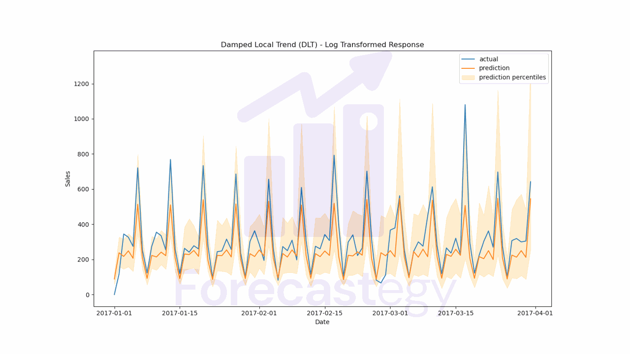
For completeness, I wanted to do the same process, but using a log transform on the target variable.
train_log = train.copy()
train_log['sales'] = np.log1p(train_log['sales'])
I will not paste the full code to be less repetitive, but now we need to exponentiate the predictions to get the original scale.
predicted_df['prediction'] = np.expm1(predicted_df['prediction'])
predicted_df['actual'] = np.expm1(predicted_df['actual'])
These were the scores on the internal validation after exponentiating the predictions:
p['prediction'] = np.expm1(p['prediction'])
p['prediction_5'] = np.expm1(p['prediction_5'])
p['prediction_95'] = np.expm1(p['prediction_95'])

{'linear': 0.17333098404592967, 'loglinear': 0.17170326730591495,
'flat': 0.17158036723838307, 'logistic': 0.1889836552516605}
I took the best option, which was flat, and trained the model with the log transform to get the final forecast.
The validation WMAPE was 25.17%, which is worse than the 20.21% we got with the original scale.
Looking at the plot, it seems the model had trouble with the peaks in sales.
The log transformation tends to devalue differences in large values, which can be a problem.
In this case, even though the log transform had better internal validation scores, the final forecast was worse.
Worth trying it anyway.
I don’t know why but it took much longer to run the log transform search.
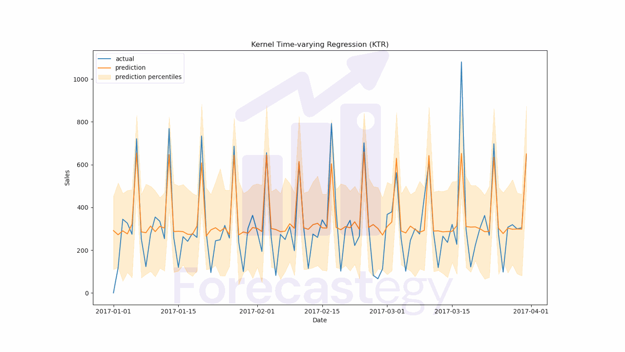
Kernel-based Time-varying Regression (KTR)
Kernel-based Time-varying Regression (KTR) is a powerful technique that combines three key innovations to help forecast time series data more effectively.
The first innovation is the use of a kernel to model regression and seasonality coefficients.
This helps constrain the number of parameters in the model, which is important because we want to avoid overfitting.
The second innovation in KTR is the use of coefficients that vary over time.
This means that instead of using the same coefficients for all time periods (like in traditional regression), we use different coefficients for each time period.
This allows our model to adapt to changes in the data over time.
For example, if we were trying to model sales data for a particular product, we might find that the coefficients that work well for one year don’t work as well for the next year, due to changes in market conditions or consumer behavior.
By allowing the coefficients to vary over time, we can capture these changes and adjust our model accordingly.
The third innovation allows us to inform the model about multiple ways seasonality affects the values we want to forecast.
For example, in retail sales data, we might see a weekly seasonality that reflects the fact that sales are higher on weekends than on weekdays.
However, there might also be an annual seasonality that reflects the fact that sales are higher during the holiday season.
This model was originally presented as a solution to marketing mix modeling, where the goal is to predict the impact of different marketing channels on sales.
from orbit.models import KTR

ktr = KTR(date_col='date',
        response_col='sales',
        seasonality=[7, 28],
        prediction_percentiles=[5, 95],
        regressor_col=['onpromotion'],
        seed=2,
        verbose=False)

ktr.fit(df=train)

p = ktr.predict(df=valid[['date', 'onpromotion']])
p = p.merge(valid, on='date', how='left')

print(wmape(p['sales'], p['prediction']))
The biggest difference here is the seasonality parameter, which is a list of integers representing the number of periods in each of the multiple seasonalities we want to model.
In this case I tried 7 and 28, but it doesn’t mean this would be better than just 7. It’s for demonstration purposes.
You can use a single value if you only want to model a single seasonality.
The validation WMAPE was 23.35%.