In this article, we will explore the use of Gaussian Processes for time series forecasting in Python, specifically using the GluonTS library.
GluonTS is an open-source toolkit for building and evaluating state-of-the-art time series models.
One of the key benefits of using Gaussian Processes for time series forecasting is that they can provide probabilistic predictions.
Instead of just predicting a point estimate for the next value in the time series, GPs can provide a distribution over possible values, allowing us to quantify our uncertainty.
This is not exclusive to GPs, so we have to take into account that it takes more time to train a GP model than a traditional model like ARIMA.
Let’s dive in!
Installing GluonTS
Before installing GluonTS, we need to install MXNet. Check out the official installation guide for more details.
Then you can install GluonTS using pip:
pip install gluonts
Preparing The Data For Gaussian Processes In GluonTS
We will use data from the City of Los Angeles website traffic dataset on Kaggle.
This dataset contains the number of user sessions for the City of Los Angeles website for each day from 2014 to 2019.
Sessions are periods of time when a user is active in a website.
Usually they are measured by looking at user activity and have a timeout after 30 minutes since the last user action.
For example, right now you are in a session on my website. If you leave the page and come back after 2 hours, you will be in a new session.
Let’s load the data and take a look at it:
import pandas as pd
import numpy as np
from matplotlib import pyplot as plt
import os

data = pd.read_csv(os.path.join(path, 'lacity.org-website-traffic.csv'),
                   parse_dates=['Date']).loc[:, ['Date', 'Device Category', 'Sessions']]
data = data.groupby(['Date', 'Device Category'], as_index=False)['Sessions'].sum()

fixes = pd.DataFrame({'Date': pd.to_datetime(['2016-12-01', '2018-10-13']),
                      'Device Category': ['tablet', 'tablet'] ,
                      'Sessions': [0, 0]})
data = pd.concat([data, fixes], axis=0, ignore_index=True)
data = data.sort_values(['Device Category', 'Date']).groupby('Device Category').apply(lambda x: x.fillna(method='ffill'))
| Date | Device Category | Sessions |
|---|---|---|
| 2014-01-01 00:00:00 | desktop | 1032805 |
| 2014-01-01 00:00:00 | mobile | 537573 |
| 2014-01-01 00:00:00 | tablet | 92474 |
| 2014-01-02 00:00:00 | desktop | 2359710 |
| 2014-01-02 00:00:00 | mobile | 607544 |
We load the data with Pandas and take only 3 columns: the date, the device category, and the number of sessions.
The original data has more detailed information about the sessions, like the browser and number of visitors, but we don’t need it for this tutorial.
We then group the data by date and device category and sum the number of sessions for each group.
Here we have 3 time series: one for desktop, one for mobile, and one for tablet.
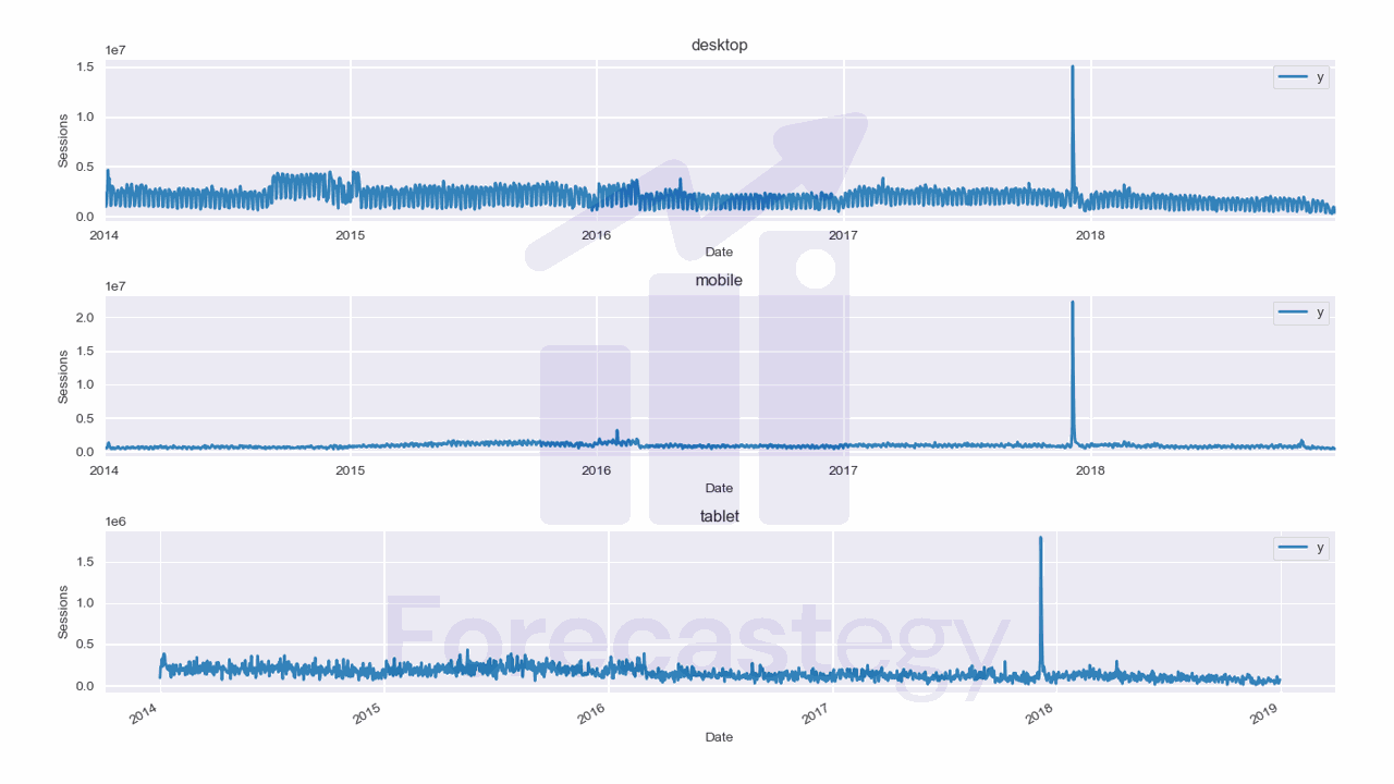
They are stacked in the long format, which means that each row represents a single observation.
This data has two observations missing for the tablet device category, so we add them manually as np.nan, then fill with the previous day value.
Now we split the data into training and validation sets with a simple time-based split:
train = data.loc[data['Date'] < '2019-01-01']
valid = data.loc[(data['Date'] >= '2019-01-01') & (data['Date'] < '2019-02-01')]
h = valid['Date'].nunique()
h is the horizon, the number of time steps we want to forecast into the future. In this case, the number of days in the validation set.
Splitting the data is important because we want to make sure that the model doesn’t overfit to the data it has seen and can’t generalize to the future.
GluonTS requires us to use a specific object for time series data.
We can easily convert our Pandas DataFrame to a GluonTS dataset using the from_long_dataframe method:
from gluonts.dataset.pandas import PandasDataset
from gluonts.dataset.multivariate_grouper import MultivariateGrouper

unique_series = train['Device Category'].nunique()
train_ds = PandasDataset.from_long_dataframe(train, target='Sessions', item_id='Device Category', timestamp='Date', freq='D')
grouper_train = MultivariateGrouper(max_target_dim=unique_series)
train_ds = grouper_train(train_ds)
This method takes in four arguments:
trainis a Pandas DataFrame containing the training data.targetis the name of the target column (the value we want to forecast)item_idis the name of the column containing unique identifiers for each time series, in case we have multiple like here.timestampis the name of the column containing the time stamps for each observationfreqis the frequency of the time series data, in this case daily.
Next, we have the grouper_train variable, which is an instance of the MultivariateGrouper class.
This class is used to group together time series data for models that implement multivariate forecasting in GluonTS.
We set the max_target_dim parameter to 3, which is the number of time series we have.
Finally, we’re passing the train_ds variable to the grouper_train() method to transform the data based on the criteria we specified earlier.
Training A Gaussian Process Model For Time Series Forecasting
We will use a flavor of Gaussian Process called GP-Copula or GPVar.
This model is a mix of a Gaussian Process and a recurrent neural network (usually LSTM).
You can find all the details in GP-Copula’s original paper.
from gluonts.mx import Trainer, GPVAREstimator

estimator = GPVAREstimator(freq='D', prediction_length=h, target_dim=unique_series, context_length=30, trainer = Trainer(ctx='gpu', epochs=5, learning_rate=1e-3))
predictor = estimator.train(train_ds)
We instantiate the GPVAREstimator class and pass in the following parameters:
freq: Frequency of the time series data. In this example, it’s set toDto indicate that the data is daily.prediction_length: Number of time steps to be predicted by the model.target_dim: Dimension of the target variable. This is typically the number of series we have. In this case, it’s set tounique_series, which is the number of unique device categories in the training data.context_length: Length of the training context. This is the number of time steps the model uses as inputs.trainer: An instance of theTrainerclass which defines how the model is trained. It specifies parameters such as the number of epochs and learning rate. In this example, it’s set to use 5 epochs, a learning rate of 1e-3, and to run on a GPU.
The learning_rate is a very important parameters that we will optimize later. It defines the step size of the optimzation algorithm used to train the model.
I found, through experience, that fixing a number of epochs and optimizing the learning rate is a good strategy to find the best model while avoiding overfitting.
If you don’t have a GPU, you can set ctx='cpu' to run the model on the CPU.
The predictor object is created by calling the train method of the estimator object, passing in the training dataset (train_ds) as an argument.
Notice that, different than the usual scikit-learn API, the train (or fit) method returns an object that can be used to generate forecasts.
Generating Forecasts
Let’s get the forecasts for the validation set:
pred = list(predictor.predict(train_ds))
The predict method takes in a dataset and returns a generator object with the forecasts.
In this case it’s a 100 by 31 by 3 array, where 100 is the number of samples it generated from the posterior distribution, 31 is the number of time steps in the validation set (the prediction horizon), and 3 is the number of unique time series.
Let’s process this data into a Pandas DataFrame to evaluate the model:
all_preds = list()
item = pred[0]
p = np.median(item.samples, axis=0).clip(0)
p10 = np.percentile(item.samples, 10, axis=0).clip(0)
p90 = np.percentile(item.samples, 90, axis=0).clip(0)
dates = pd.date_range(start=item.start_date.to_timestamp(), periods=len(p), freq='D')

for name, q in [('p50', p), ('p10', p10), ('p90', p90)]:
    wide_p = pd.DataFrame({'Date': dates})
    for i, device in enumerate(train_['Device Category'].unique()):
        wide_p[device] = q[:, i]
    wide_p = wide_p.melt(id_vars='Date', var_name='Device Category', value_name=name)
    all_preds.append(wide_p.set_index(['Date', 'Device Category']))

all_preds = pd.concat(all_preds, axis=1).reset_index()
all_preds = all_preds.merge(valid, on=['Date', 'Device Category'], how='left')

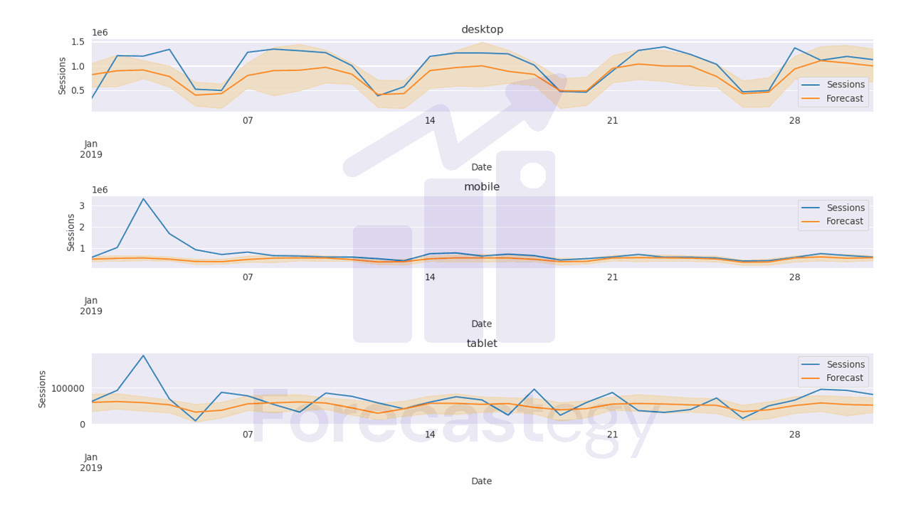
The code above computes the median, 10th percentile, and 90th percentile of the predicted values.
It uses numpy to compute these percentiles along the samples axis of the predicted values array.
The for loop then creates a Pandas dataframe with the date range and the predicted values for each device category as the columns.
The melt function is used to unpivot the dataframe, converting the device categories to a single column, and the values to a separate column. The resulting dataframe for each percentile is then appended to the all_preds list.
After computing the predicted values for each percentile, the code concatenates the dataframes in all_preds along the columns axis, resulting in a single dataframe with dates, columns for each percentile (p50, p10, p90) and device category.
| Date | Device Category | p50 | p10 | p90 | Sessions |
|---|---|---|---|---|---|
| 2019-01-01 00:00:00 | desktop | 1.06014e+06 | 625134 | 1.43136e+06 | 315674 |
| 2019-01-02 00:00:00 | desktop | 1.06372e+06 | 643280 | 1.47342e+06 | 1209157 |
| 2019-01-03 00:00:00 | desktop | 986666 | 660598 | 1.32867e+06 | 1199978 |
| 2019-01-04 00:00:00 | desktop | 892633 | 734292 | 1.14378e+06 | 1339970 |
| 2019-01-05 00:00:00 | desktop | 445984 | 282950 | 591550 | 516879 |
We merge the dataframe with the validation data based on the date and device category columns so it’s straightforward to compute the pinball loss.
Evaluating The Model
The Pinball loss is a commonly used metric in time series forecasting that measures the deviation of the predicted quantiles from the actual values at a specific quantile level.
from sklearn.metrics import mean_pinball_loss
for q in [0.1, 0.5, 0.9]:
    print(f'pinball loss at {q}: {mean_pinball_loss(all_preds["Sessions"], all_preds[f"p{int(q*100)}"], alpha=q)}')
The code imports the mean_pinball_loss function from scikit-learn.
It then calculates the pinball loss for quantiles of 0.1, 0.5, and 0.9 using a for loop.
Inside the loop, the function is called with the following arguments: the actual values of sessions (all_preds["Sessions"]), the predicted values for the corresponding quantile (all_preds[f"p{int(q*100)}"]), and the value of alpha (which is the quantile).
The final numbers are:
- pinball loss at 0.1: 33952.08
- pinball loss at 0.5: 87465.95
- pinball loss at 0.9: 68380.55
Let’s see if we can improve the model by optimizing the hyperparameters.
Optimizing The Hyperparameters Of The Gaussian Process With Optuna
We will use Optuna to optimize the hyperparameters of the Gaussian Process model.
This is a very simple library that uses Tree-structured Parzen Estimator (TPE) to optimize the hyperparameters of the model.
We just need to encapsulate the code that trains the model in a function that takes a trial object as an argument.
The trial object is a single step of the optimization process.
The function returns a list of values, as we want to optimize the pinball loss at quantiles of 0.1, 0.5, and 0.9.
def objective(trial):
    context_length = trial.suggest_int('context_length', 7, 400)
    learning_rate = trial.suggest_loguniform('learning_rate', 1e-5, 1e-1)
    num_layers = trial.suggest_int('num_layers', 1, 4)
    num_cells = trial.suggest_int('num_cells', 8, 128)
    cell_type = trial.suggest_categorical('cell_type', ['lstm', 'gru'])
    dropout_rate = trial.suggest_uniform('dropout_rate', 0.1, 0.9)
    rank = trial.suggest_int('rank', 1, 3)


    estimator = GPVAREstimator(freq='D', prediction_length=h, target_dim=unique_series,
                               context_length=context_length, num_layers=num_layers,
                               num_cells=num_cells, cell_type=cell_type, dropout_rate=dropout_rate,
                               rank=rank,  trainer = Trainer(ctx='gpu', epochs=5, learning_rate=learning_rate))
    predictor = estimator.train(train_ds)
    pred = list(predictor.predict(train_ds))

    all_preds = list()
    item = pred[0]
    p = np.median(item.samples, axis=0).clip(0)
    p10 = np.percentile(item.samples, 10, axis=0).clip(0)
    p90 = np.percentile(item.samples, 90, axis=0).clip(0)
    dates = pd.date_range(start=item.start_date.to_timestamp(), periods=len(p), freq='D')
    for name, q in [('p50', p), ('p10', p10), ('p90', p90)]:
        wide_p = pd.DataFrame({'Date': dates})
        for i, device in enumerate(train_['Device Category'].unique()):
            wide_p[device] = q[:, i]
        wide_p = wide_p.melt(id_vars='Date', var_name='Device Category', value_name=name)
        all_preds.append(wide_p.set_index(['Date', 'Device Category']))

    all_preds = pd.concat(all_preds, axis=1).reset_index()
    all_preds = all_preds.merge(valid, on=['Date', 'Device Category'], how='left')

    return [mean_pinball_loss(all_preds["Sessions"], all_preds[f"p{int(q*100)}"], alpha=q) for q in [0.1, 0.5, 0.9]]
We define the hyperparameters search space using the suggest_* methods of the trial object.
These methods will sample a value from the specified range or distribution.
Here is a breakdown of each parameter:
context_length: the number of time steps in the past that the model should use to make a prediction about the future. I set a range from 7 to 400 so we can test very short and very long windows.learning_rate: the step size at which the model adjusts its weights during training. A small learning rate can lead to slower convergence, while a large learning rate can lead to overshooting the optimal weights. A good rule of thumb is to use a log-uniform distribution between 1e-5 and 1e-1.num_layers: the number of layers in the RNN model. A deeper model can capture more complex patterns in the data, but can also be prone to overfitting. Let’s try values between 1 and 4. More layers than that are usually not necessary for time series forecasting.num_cells: the number of units or neurons in each layer of the model. A number between 8 and 128 should be enough.cell_type: the type of recurrent neural network (RNN) cell to use in the model. This can be either Long Short-Term Memory (LSTM) or Gated Recurrent Unit (GRU). These are both popular choices for time series forecasting.dropout_rate: the rate at which to randomly drop out units in the model during training to prevent overfitting. A good range is between 0.1 and 0.9.rank: the rank of the distribution that will be used to sample the predictions. Default is 2, but let’s try values between 1 and 3.
The rest of the code is similar to the previous example.
To run the optimization, we just need to call the optimize method of the study object.
import optuna
study = optuna.create_study(directions=['minimize', 'minimize', 'minimize'])
study.optimize(objective, n_trials=20, timeout=900)
We set the directions of each returned value to minimize because we want to minimize the pinball losses at all quantiles.
n_trials is the number of steps to run. 20 is usually a good number to start with. 30 is enough for most cases.
The timeout argument is the maximum time in seconds to run the optimization.
After a long time, you can get the best hyperparameters and the corresponding pinball losses.
The attribute study.best_trials returns a list of the best trials, meaning the trials that returned the lowest values for any of the objectives.
After inspecting it, I found the second element of the returned list to be the minimum for 2 of the 3 objectives, so I picked it.
best_trial = study.best_trials[1]
best_trial.params
{'context_length': 270,
 'learning_rate': 0.013101512029143874,
 'num_layers': 1,
 'num_cells': 84,
 'cell_type': 'lstm',
 'dropout_rate': 0.16228795203947746,
 'rank': 2}
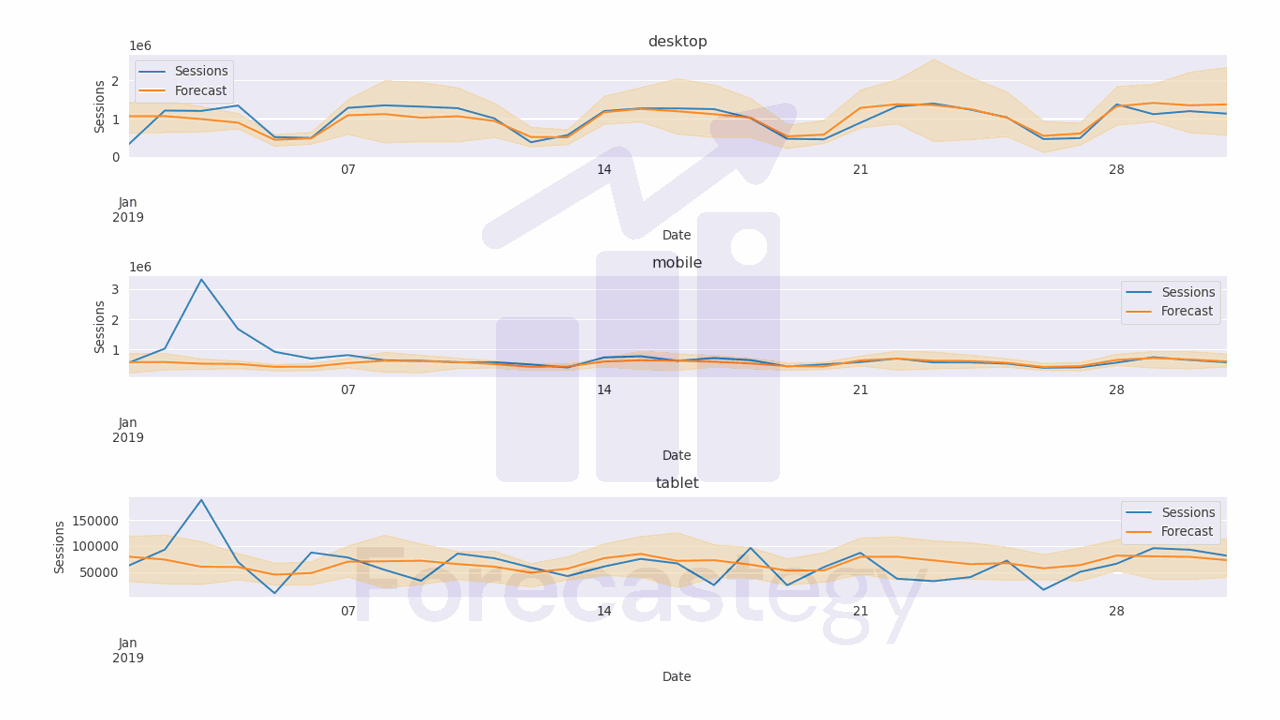
To get the corresponding values for the objectives, we can call the values attribute of the best_trial object.
best_trial.values
[31605.068581359206, 64329.63781081989, 69049.05124747986]
The model improved, but I found it takes too long to reach a good solution compared to alternatives like CNNs, “pure” LSTMs or Kalman filters