The Kalman Filter is a state-space model that estimates the state of a dynamic system based on a series of noisy observations.
It uses a feedback mechanism called the Kalman gain to adjust the weight given to predicted and observed values based on their relative uncertainties.
It has been widely used in various fields such as finance, aerospace, and robotics.
In this tutorial, you will learn how to easily use the Kalman Filter for time series forecasting in Python.
We use Darts, which is a powerful and user-friendly Python library for time series forecasting that offers a range of models, tools, and utilities.
It provides a simple interface for loading, preprocessing, and modeling time series data, making it an ideal choice for beginners and experts alike.
Let’s get started!
What Is A Kalman Filter?
Picture this: suppose you’re trying to find the location of a moving object, like your friend riding their bike.
Your GPS tracker, however, is not very accurate and sometimes gives you wrong location estimates.
Wouldn’t it be fantastic if there was some magical way to predict your friend’s true position?
That’s where Kalman Filters come in!
Although not magical, they are a set of mathematical equations that help estimate the true state of dynamic systems (like moving objects) by factoring in measurement uncertainties and noise.
In other words, they find the most likely position or state of a system based on noisy or incomplete data.
For a very noisy time series, like stock prices, the Kalman Filter can be used to smooth out the noise, get closer to the “true” price, and make predictions.
When Should You Use A Kalman Filter?
Kalman Filters are perfect for time series forecasting in dynamic systems that require real-time tracking or estimation.
They can especially come in handy when your forecasting relies on noisy or imprecise data, like inputs from sensors such as GPS or accelerometers.
For instance, imagine you want to predict the future position of a moving object based on noisy sensor data.
A Kalman Filter will help refine those readings and provide a more accurate forecast of the object’s future state.
Moreover, Kalman Filters are an excellent choice when you need to update your predictions as new data comes in.
They can adapt seamlessly to the continuous inflow of data, adjusting your forecast in real-time while accounting for uncertainties in the measurements.
However, there are times when using Kalman Filters may not be ideal:
- Static systems: If your system doesn’t change over time (i.e., it’s not dynamic), or if your measurements are already very accurate, then there’s no need for the extra effort of filtering.
- Complex, nonlinear behavior: When your system exhibits nonlinear behavior, a Kalman Filter might not be sufficient. In such cases, consider exploring other options like Particle Filters, which are specifically designed to handle intricate situations.
Kalman Filter Equations
Let’s dive into the Kalman Filter equations and what each symbol means.
The Kalman Filter consists of two main steps: the predict step and the update step.
First, here are the equations:
- Predict step:
- State prediction: $x_{t|t-1} = F_t x_{t-1|t-1} + B_t u_t$
- Uncertainty prediction: $P_{t|t-1} = F_t P_{t-1|t-1} F_t^T + Q_t$
- Update step:
- Kalman gain: $K_t = P_{t|t-1} H_t^T (H_t P_{t|t-1} H_t^T + R_t)^{-1}$
- State update: $x_{t|t} = x_{t|t-1} + K_t (z_t - H_t x_{t|t-1})$
- Uncertainty update: $P_{t|t} = (I - K_t H_t) P_{t|t-1}$
Let’s understand these symbols thinking about a stock price prediction problem.
(Not financial advice! I am not responsible for any losses you may incur.)
In the stock price modeling context, the goal of the Kalman Filter would be to estimate the underlying stock price trend, factoring in the influence of external factors and accounting for the noise in the recorded prices.
- $x$: The state vector, which represents the true state of the stock price that we want to estimate.
- $t$: The time step index, corresponding to different trading days or time periods.
- $F_t$: The state transition matrix, which models how the stock price evolves from time step $t-1$ to $t$ without taking into account external factors (e.g., market trends or news events).
- $B_t$: The control input matrix, used to incorporate the effect of any external factors $u_t$ (e.g., financial news or announcements affecting the stock price).
- $u_t$: The control input vector, containing the external factors impacting the stock price.
- $P$: The uncertainty (covariance) matrix, which quantifies our uncertainty about the estimated stock price.
- $Q_t$: The process noise covariance matrix, representing the estimation error caused by our simplified model of the stock price dynamics.
- $H_t$: The observation matrix, which models how the true stock price is transformed into the observed stock price (e.g., recorded price at market close).
- $K_t$: The Kalman gain, which determines how much we trust the new observation (e.g., daily closing price) relative to our prediction.
- $z_t$: The observation (measurement) vector, containing the recorded stock prices.
- $R_t$: The observation noise covariance matrix, representing the measurement noise in the observed stock prices (e.g., fluctuations during a trading day).
- $I$: The identity matrix.
This can help generate more accurate forecasts and inform investment decisions.
Now, let’s walk through the step-by-step filtering process:
- Predict the stock price ($x_{t|t-1}$) and uncertainty ($P_{t|t-1}$) at time step $t$ based on the previous stock price and uncertainty at time step $t-1$.
- Obtain a new recorded stock price ($z_t$) at time step $t$.
- Calculate the Kalman gain ($K_t$) to determine how much trust to place in the new recorded price compared to our prediction.
- Update the stock price estimate ($x_{t|t}$) by combining the predicted price, Kalman gain, and new recorded price.
- Update the uncertainty estimate ($P_{t|t}$) to reflect the reduced uncertainty after incorporating the new recorded stock price.
This process is repeated at each time step, allowing the Kalman Filter to continuously predict and update the state estimate and uncertainty with the incoming measurements.
To estimate the internal matrices from data, Darts uses the N4SID algorithm.
Installing Darts
You can install Darts using pip:
pip install darts
Or, if you prefer to use conda:
conda install -c conda-forge -c pytorch u8darts-all
If you run into any issues, please refer to the Darts installation guide.
Preparing Time Series Data For Kalman Filters
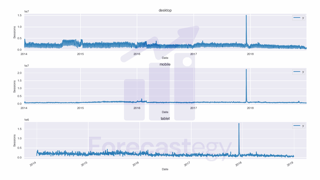
We will use data from the City of Los Angeles website traffic dataset on Kaggle.
This dataset contains the number of user sessions for the City of Los Angeles website for each day from 2014 to 2019.
Sessions are periods of time when a user is active in a website.
Usually they are measured by looking at user activity and have a timeout after 30 minutes since the last user action.
For example, right now you are in a session on my website. If you leave the page and come back after 2 hours, you will be in a new session.
Let’s load the data and take a look at it:
import pandas as pd
import numpy as np
from matplotlib import pyplot as plt
import os

data = pd.read_csv(os.path.join(path, 'lacity.org-website-traffic.csv'),
                   parse_dates=['Date']).loc[:, ['Date', 'Device Category', 'Sessions']]
data = data.groupby(['Date', 'Device Category'], as_index=False)['Sessions'].sum()

fixes = pd.DataFrame({'Date': pd.to_datetime(['2016-12-01', '2018-10-13']),
                      'Device Category': ['tablet', 'tablet'] ,
                      'Sessions': [0, 0]})
data = pd.concat([data, fixes], axis=0, ignore_index=True)
| Date | Device Category | Sessions |
|---|---|---|
| 2014-01-01 00:00:00 | desktop | 1032805 |
| 2014-01-01 00:00:00 | mobile | 537573 |
| 2014-01-01 00:00:00 | tablet | 92474 |
| 2014-01-02 00:00:00 | desktop | 2359710 |
| 2014-01-02 00:00:00 | mobile | 607544 |
We load the data with Pandas and take only 3 columns: the date, the device category, and the number of sessions.
The original data has more detailed information about the sessions, like the browser and number of visitors, but we don’t need it for this tutorial.
We then group the data by date and device category and sum the number of sessions for each group.
Here we have 3 time series: one for desktop, one for mobile, and one for tablet.

They are stacked in the long format, which means that each row represents a single observation.
This data has two points missing for the tablet device category, so we add them manually as np.nan, then fill with the previous day value.
Now we split the data into training and validation sets with a simple time-based split:
train = data.loc[data['Date'] < '2019-01-01']
valid = data.loc[(data['Date'] >= '2019-01-01') & (data['Date'] < '2019-04-01')]
h = valid['Date'].nunique()
h is the horizon, the number of time steps we want to forecast into the future. In this case, the number of days in the validation set.
Splitting the data is important because we want to make sure that the model doesn’t overfit to the data it has seen and can’t generalize to the future.
Darts requires us to use the TimeSeries class to represent time series data.
from darts import TimeSeries

series_names = train['Device Category'].unique()
train_series = TimeSeries.from_group_dataframe(train, time_col='Date', value_cols=['Sessions'], group_cols=['Device Category'], freq='D', fill_missing_dates=True, fillna_value=0.)
We create a list with the device categories names so that we can identify the time series later.
Then we use the from_group_dataframe method to create a list of TimeSeries objects from the training data.
There was a bug in version 0.23.1 of Darts that caused this operation to return a ValueError.
The developers told this will be fixed in the next release, so if the version available on PyPI or conda-forge is still 0.23.1, you can install the latest version from GitHub:
pip install git+https://github.com/unit8co/darts
The from_group_dataframe method takes:
- the dataframe with the data
time_colis the name of the column with the datevalue_colsis the name of the column with the values we want to forecastgroup_colsis the name of the column with the group names that identify each time seriesfreqis the frequency of the datafill_missing_datesis a boolean that tells Darts to insert records for missing dates withnp.nanvaluesfillna_valueis the value to use to fill the missing values in the time series
This method returns a list of TimeSeries objects, one for each group. So each time series is treated as a separate entity.
If you have only one time series, you can use the from_dataframe method instead.
Training The Kalman Filter For Time Series Forecasting
We will use the KalmanForecast class from Darts to train the Kalman Filter.
from darts.models import KalmanForecaster
As we have more than one time series, we will train a separate model for each one inside a loop.
preds = list()
for i, series in enumerate(train_series):
    model = KalmanForecaster(dim_x=100)
    model.fit(series=series)
    p = model.predict(h).pd_dataframe().reset_index()
    p['Device Category'] = series_names[i]
    preds.append(p)
preds = pd.concat(preds, axis=0, ignore_index=True).rename(columns={'Sessions': 'Predicted'})
The KalmanForecaster class takes the dim_x parameter, which is the dimension of the state vector.
I think about it as the size of an internal representation of the time series.
From a practitioner’s point of view, this is a hyperparameter that you can tune to get better results.
In this case I found a value of 100 to be good for this dataset after evaluating the MAPE of a few different values in the validation set.
After creating the model, we fit it to the training data.
Then we use the predict method to make predictions for the validation set.
This method takes the horizon, which is the number of steps to forecast.
The method pd_dataframe converts the TimeSeries object to a Pandas dataframe and we add a column to identify the series that the prediction belongs to.
Finally, we append the predictions to a list and concatenate them into a single dataframe.
| Date | Predicted | Device Category | Sessions |
|---|---|---|---|
| 2019-01-01 00:00:00 | 1.00565e+06 | desktop | 315674 |
| 2019-01-02 00:00:00 | 1.07962e+06 | desktop | 1209157 |
| 2019-01-03 00:00:00 | 936168 | desktop | 1199978 |
| 2019-01-04 00:00:00 | 850586 | desktop | 1339970 |
| 2019-01-05 00:00:00 | 166220 | desktop | 516879 |
To know how well the model is doing, we can calculate the MAPE of the predictions.
preds = preds.merge(valid, on=['Date', 'Device Category'], how='left')

from sklearn.metrics import mean_absolute_percentage_error
mean_absolute_percentage_error(preds['Sessions'], preds['Predicted'])
I merged the predictions dataframe with the validation set to make it easier to calculate the MAPE and then used the mean_absolute_percentage_error function from scikit-learn.
This model has a MAPE of 31.47% on the validation set. Let’s visualize the forecast.
fig,ax = plt.subplots(3,1,figsize=(1280/96, 720/96), dpi=96)
preds_ = preds[preds['Date'] >= '2019-01-10']
for ax_, device in enumerate(preds_['Device Category'].unique()):
    p_ = preds_.loc[preds_['Device Category'] == device]
    p_.rename(columns={'Sessions': 'Actual'}, inplace=True)
    p_.plot(x='Date', y=['Predicted', 'Actual'], ax=ax[ax_], title=device)
    ax[ax_].set_xlabel('Date')
    ax[ax_].set_ylabel('Sessions')
fig.tight_layout()
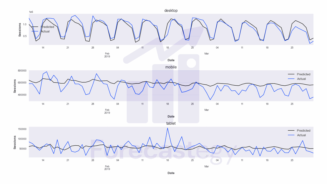
I ploted it from January 10th to the end of the validation set because there is a peak in the data that makes it hard to visualize the forecast if we include the dates before that.
The model is doing well for the desktop category, but it’s not doing so well for the mobile and tablet categories.
If this happens in your data, you may try other approaches for these series like scikit-learn, ARIMA or even a simple Seasonal Naive model.
Kalman Filter Forecasting With Prediction Intervals
The predict method of the KalmanForecaster can return a probabilistic forecast too.
Probabilistic forecasts tend to be very useful in practice because they give you an idea of how confident you can be in the forecast.
We just need to add the num_samples argument to it and use the quantile_df method to get any quantiles we want.
from darts.models import KalmanForecaster

preds = list()
for i, series in enumerate(train_series):
    model = KalmanForecaster(dim_x=100)
    model.fit(series=series)
    p = model.predict(h, num_samples=100)
    p = [p.quantile_df(q) for q in [0.05, 0.5, 0.95]]
    p = pd.concat(p, axis=1).reset_index()
    p['Device Category'] = series_names[i]
    preds.append(p)
preds = pd.concat(preds, axis=0, ignore_index=True)
preds = preds.merge(valid, on=['Date', 'Device Category'], how='left')
Now, instead of a single prediction, we get a dataframe with the 5th, 50th and 95th percentiles of the forecast.
We can then plot it.
fig,ax = plt.subplots(3,1,figsize=(1280/96, 720/96), dpi=96)
preds_ = preds[preds['Date'] >= '2019-01-10']
for ax_, device in enumerate(preds_['Device Category'].unique()):
    p_ = preds_.loc[preds_['Device Category'] == device]
    p_.rename(columns={'Sessions': 'Actual', 'Sessions_0.5': 'Predicted'}, inplace=True)
    ax[ax_].fill_between(p_['Date'], p_['Sessions_0.05'], p_['Sessions_0.95'], alpha=0.2)
    p_.plot(x='Date', y=['Predicted', 'Actual'], ax=ax[ax_], title=device)
    ax[ax_].set_xlabel('Date')
    ax[ax_].set_ylabel('Sessions')
fig.tight_layout()
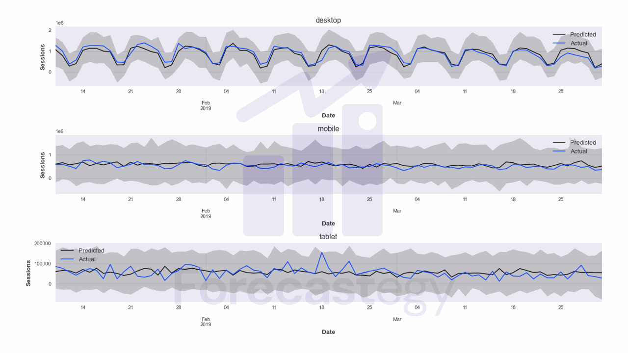
The grey area represents the prediction interval.
To evaluate quantile forecasts, we can use the Pinball Loss, which is basically the mean absolute error adapted to quantile forecasts.
from sklearn.metrics import mean_pinball_loss
for q in [0.05, 0.5, 0.95]:
    print(f'Pinball loss at {q}: {mean_pinball_loss(preds["Sessions"], preds[f"Sessions_{q}"])}')
These are the results at the 5th, 50th and 95th percentiles:
- Pinball loss at 0.05: 264936.47
- Pinball loss at 0.5: 51491.41
- Pinball loss at 0.95: 270084.79
Lower is better.