In this tutorial, I will explain two (and a half) methods to generate multi-step forecasts using time series data.
They are the recursive or autoregressive method, the direct method, and a variant of the direct method with a single model.
Preparing the Data
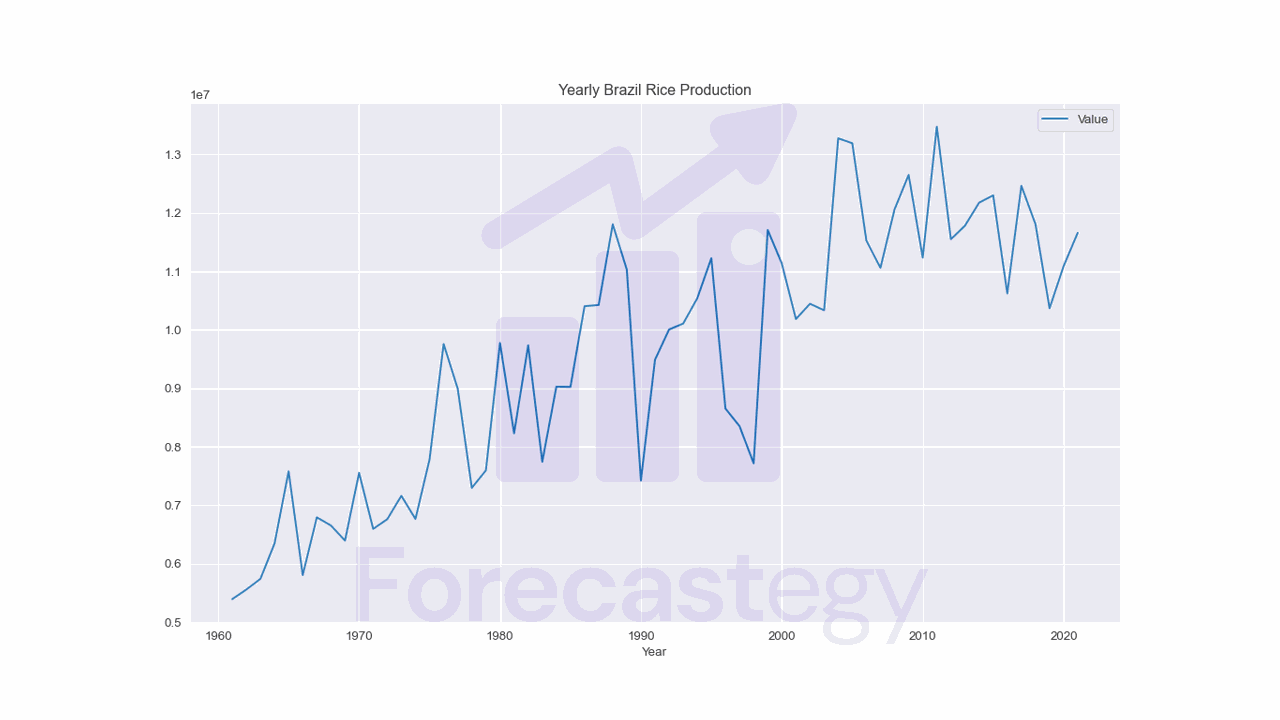
We will use a dataset containing information about yearly rice production.
import pandas as pd
import numpy as np
import os

data = pd.read_csv(os.path.join(path, 'rice production across different countries from 1961 to 2021.csv'))
data = data[data['Area'] == 'Brazil'].copy()

train = data[data['Year'] < 2017].copy()
valid = data[data['Year'] >= 2017].copy()
| Area | Year | Unit | Value | Flag | Flag Description |
|---|---|---|---|---|---|
| Brazil | 2005 | tonnes | 1.31929e+07 | A | Official figure |
| Brazil | 2006 | tonnes | 1.15267e+07 | A | Official figure |
| Brazil | 2007 | tonnes | 1.10607e+07 | A | Official figure |
| Brazil | 2008 | tonnes | 1.20615e+07 | A | Official figure |
| Brazil | 2009 | tonnes | 1.26511e+07 | A | Official figure |

It contains very simple time series data for yearly rice production in many countries.
We will use only data from Brazil to simplify the problem and try to predict the next 5 years.
Always split your data into training and validation sets before doing anything else. This is to avoid data leakage.
Recursive Or Autoregressive Method In Pure Python
The first (and most popular) method to generate multi-step forecasts is the recursive or autoregressive method.
This method consists of training a machine learning model, in this case, a linear regression model, using lagged values of the time series as input features and one step ahead as the target variable.
After training the model, we use the last lagged values of the training set to predict the next value.
Then, we shift the lagged values by one position, removing the oldest one and adding the predicted value as if it were the newest one, and repeat the process for the next forecast.
lag = 3
x = list()
y = list()
for t in range(lag, len(train)):
    x.append(train['Value'].iloc[t-lag:t].values)
    y.append(train['Value'].iloc[t])
In this first block of code, we define the lag parameter, which determines the number of previous values used as input features.
Then, we create two empty lists, x and y, to store the input features and target values, respectively.
We loop over the training set to create rows with the sequences of lagged values as features and the next value as the target.
This is what the result looks like:
| t-2 | t-1 | t | t+1 |
|---|---|---|---|
| 1.0446e+07 | 1.03346e+07 | 1.3277e+07 | 1.31929e+07 |
| 1.03346e+07 | 1.3277e+07 | 1.31929e+07 | 1.15267e+07 |
| 1.3277e+07 | 1.31929e+07 | 1.15267e+07 | 1.10607e+07 |
| 1.31929e+07 | 1.15267e+07 | 1.10607e+07 | 1.20615e+07 |
| 1.15267e+07 | 1.10607e+07 | 1.20615e+07 | 1.26511e+07 |
You can see that t+1 always becomes t in the next row and we drop the oldest value (t-2).
After that, it’s straightforward to train any machine learning model using the data we just created and make predictions.
from sklearn.linear_model import LinearRegression

model = LinearRegression()
model.fit(x, y)

p = np.zeros(len(valid))
x_ = train['Value'].iloc[-lag:].values
for t in range(len(valid)):
    p[t] = model.predict([x_])
    x_ = np.roll(x_, -1)
    x_[-1] = p[t]

We initialize the p array to store the predictions with the size of our horizon, which is the number of steps we want to forecast (5 in this case, or the size of the validation set).
Then, we initialize the input vector x_ with the most recent values of the training set.
Inside the loop we predict the next value, store it in the p array, and shift the values of x_ one position, removing the oldest one and adding the predicted value as if it were the newest one.
We can do this indefinitely, but we need to be careful with the accumulated error.
Recursive Or Autoregressive Method With SKForecast
In practice, it’s much easier to use a library like skforecast to do this.
The example above was intended for you to learn how the recursive method works, but in practice, use the library.
from skforecast.ForecasterAutoreg import ForecasterAutoreg

train_ = train[['Year', 'Value']].copy().set_index('Year').squeeze()

forecaster = ForecasterAutoreg(regressor=LinearRegression(),
                                     lags=lag)

forecaster.fit(y=train_)

predictions = forecaster.predict(steps=5)
The ForecasterAutoreg class requires a Pandas Series, so we create a copy of the training set and set the index to the Year column.
Then, we create an instance of the ForecasterAutoreg class and pass the LinearRegression model and the number of lags as parameters.
After training the model, we use the predict method to make the forecast for as many steps as we want.
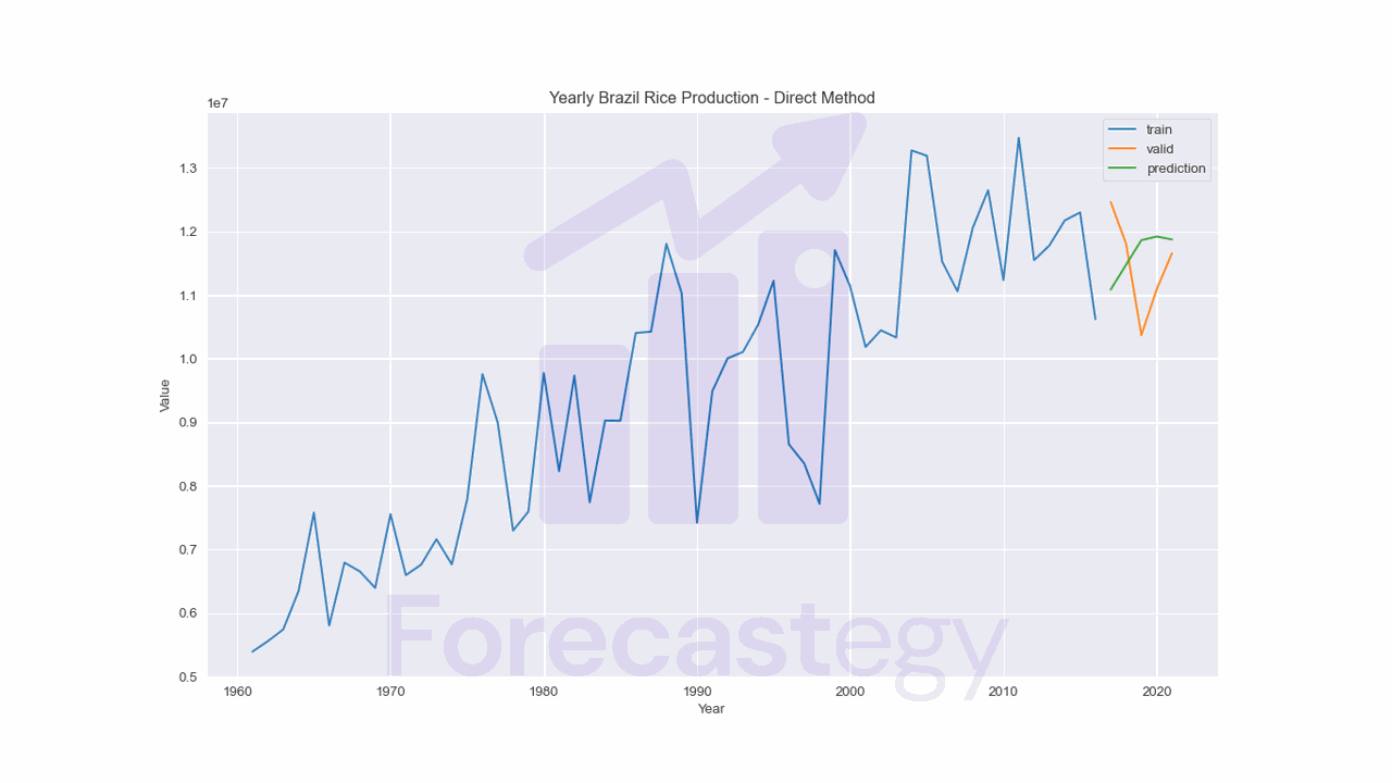
Direct Method
This method consists of training a machine learning model to directly predict the target variable h steps ahead.
Instead of creating a model to predict the next value (t+1), we create a model passing the value at the step t+h as the target variable.
from sklearn.linear_model import LinearRegression

lag = 3
p = np.zeros(len(valid))
for h in range(len(valid)):
    x = list()
    y = list()
    for t in range(lag, len(train)-h):
        x.append(train['Value'].iloc[t-lag:t].values)
        y.append(train['Value'].iloc[t+h])

    model = LinearRegression()
    model.fit(x, y)

    x_ = train['Value'].iloc[-lag:].values
    p[h] = model.predict([x_])
| t-2 | t-1 | t | t+h |
|---|---|---|---|
| 1.01073e+07 | 1.05408e+07 | 1.12261e+07 | 1.11346e+07 |
| 1.05408e+07 | 1.12261e+07 | 8.65233e+06 | 1.01842e+07 |
| 1.12261e+07 | 8.65233e+06 | 8.35166e+06 | 1.0446e+07 |
| 8.65233e+06 | 8.35166e+06 | 7.71609e+06 | 1.03346e+07 |
| 8.35166e+06 | 7.71609e+06 | 1.17097e+07 | 1.3277e+07 |
| 7.71609e+06 | 1.17097e+07 | 1.11346e+07 | 1.31929e+07 |
| 1.17097e+07 | 1.11346e+07 | 1.01842e+07 | 1.15267e+07 |
| 1.11346e+07 | 1.01842e+07 | 1.0446e+07 | 1.10607e+07 |
| 1.01842e+07 | 1.0446e+07 | 1.03346e+07 | 1.20615e+07 |
| 1.0446e+07 | 1.03346e+07 | 1.3277e+07 | 1.26511e+07 |
Notice the difference in the y list: we are using the value at the step t+h instead of t+1.
The method name is direct because we are training a model to directly predict the target variable h steps ahead.
The downside is that we need to train a model for each step ahead, which can be computationally expensive.
After we have the models, we can use them to make predictions.
Here we are using the same input vector x_, it’s the model that changes, as each model is trained to predict a different step ahead.
Direct Method With SKForecast
Again, in practice, I recommend using a library like SKForecast to save time and avoid mistakes.
from skforecast.ForecasterAutoregDirect import ForecasterAutoregDirect

train_ = train[['Year', 'Value']].copy().set_index('Year').squeeze()

forecaster = ForecasterAutoregDirect(regressor=LinearRegression(),
                lags=lag, steps=len(valid))

forecaster.fit(y=train_)

predictions = forecaster.predict()
After creating the Pandas Series from the training set, we create an instance of the ForecasterAutoregDirect class and pass the LinearRegression model, the number of lags, and the number of steps we want to predict.
Remember that one model will be trained for each step ahead, so the number of steps is the same as the number of models.
To get the predictions, we simply use the predict method.
Direct Method With a Single Model
This is a variation of the direct method that we can use with models that can predict multiple targets at once].
from sklearn.linear_model import LinearRegression

lag = 3
p = np.zeros(len(valid))
h = len(valid)

x = list()
y = list()
for i in range(lag, len(train)-h+1):
    x.append(train['Value'].iloc[i-lag:i].values)
    y.append(train['Value'].iloc[i:i+h].values)

model = LinearRegression()
model.fit(x, y)

x_ = train['Value'].iloc[-lag:].values
p = model.predict([x_])
| t-2 | t-1 | t | t+1 | t+2 | t+3 | t+4 | t+5 |
|---|---|---|---|---|---|---|---|
| 1.01073e+07 | 1.05408e+07 | 1.12261e+07 | 8.65233e+06 | 8.35166e+06 | 7.71609e+06 | 1.17097e+07 | 1.11346e+07 |
| 1.05408e+07 | 1.12261e+07 | 8.65233e+06 | 8.35166e+06 | 7.71609e+06 | 1.17097e+07 | 1.11346e+07 | 1.01842e+07 |
| 1.12261e+07 | 8.65233e+06 | 8.35166e+06 | 7.71609e+06 | 1.17097e+07 | 1.11346e+07 | 1.01842e+07 | 1.0446e+07 |
| 8.65233e+06 | 8.35166e+06 | 7.71609e+06 | 1.17097e+07 | 1.11346e+07 | 1.01842e+07 | 1.0446e+07 | 1.03346e+07 |
| 8.35166e+06 | 7.71609e+06 | 1.17097e+07 | 1.11346e+07 | 1.01842e+07 | 1.0446e+07 | 1.03346e+07 | 1.3277e+07 |
| 7.71609e+06 | 1.17097e+07 | 1.11346e+07 | 1.01842e+07 | 1.0446e+07 | 1.03346e+07 | 1.3277e+07 | 1.31929e+07 |
| 1.17097e+07 | 1.11346e+07 | 1.01842e+07 | 1.0446e+07 | 1.03346e+07 | 1.3277e+07 | 1.31929e+07 | 1.15267e+07 |
| 1.11346e+07 | 1.01842e+07 | 1.0446e+07 | 1.03346e+07 | 1.3277e+07 | 1.31929e+07 | 1.15267e+07 | 1.10607e+07 |
| 1.01842e+07 | 1.0446e+07 | 1.03346e+07 | 1.3277e+07 | 1.31929e+07 | 1.15267e+07 | 1.10607e+07 | 1.20615e+07 |
| 1.0446e+07 | 1.03346e+07 | 1.3277e+07 | 1.31929e+07 | 1.15267e+07 | 1.10607e+07 | 1.20615e+07 | 1.26511e+07 |

Notice that y became a matrix with h columns, one for each step ahead.
It’s the simplest way in terms of code, as we only need to train a single model and can use the same input vector x_ for all predictions.
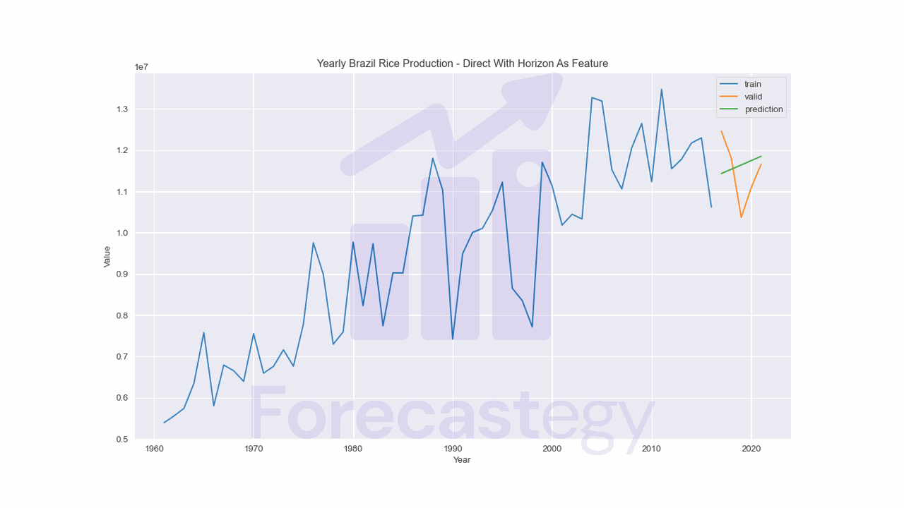
Direct Method With Horizon As A Feature
This is another variation of the direct method that we can use with models that predict only a single target at a time (like XGBoost).
I saw it on this Kaggle Days presentation and decided to add it here.
It uses an old trick that I have used a lot to transform a multiclass/multilabel problem into a binary classification problem.
For example, if we have 10 classes, we can create a feature that takes the value of the class that we want to predict and the target becomes a binary indicator for “does this observation belong to this class?”
In the case of regression/time series forecasting, we add the horizon as a feature and stack multiple rows for the same target.
lag = 3
p = np.zeros(len(valid))
x = list()
y = list()
for h in range(len(valid)):
    for t in range(lag, len(train)-h):
        x_ = np.zeros(lag+1)
        x_[:-1] = train['Value'].iloc[t-lag:t].values
        x_[-1] = h
        x.append(x_)
        y.append(train['Value'].iloc[t+h])

model = LinearRegression()
model.fit(x, y)
| t-2 | t-1 | t | h | t+h |
|---|---|---|---|---|
| 1.3277e+07 | 1.31929e+07 | 1.15267e+07 | 0 | 1.10607e+07 |
| 1.03346e+07 | 1.3277e+07 | 1.31929e+07 | 1 | 1.10607e+07 |
| 1.0446e+07 | 1.03346e+07 | 1.3277e+07 | 2 | 1.10607e+07 |
| 1.01842e+07 | 1.0446e+07 | 1.03346e+07 | 3 | 1.10607e+07 |
| 1.11346e+07 | 1.01842e+07 | 1.0446e+07 | 4 | 1.10607e+07 |
Notice that we have 5 rows for each target, one for each step of the horizon, and now we get the h column indicating which step we are predicting.
Here the next step is h=0 and so on.
To forecast we just need to change the h value in the input vector for each step.
x_ = np.zeros(lag+1)
x_[:-1] = train['Value'].iloc[-lag:].values
for h in range(len(valid)):
    x_[-1] = h
    p[h] = model.predict([x_])
Which Multi-Step Forecasting Method Is Best?
There is no way to know which method is best without trying them all in your problem.
I have seen people win forecasting competitions with all of them.
It’s good to go beyond accuracy and look at other metrics, such as the time it takes to train the models and make predictions.
The direct method requires multiple models, which means more storage and time to train and predict.
The recursive method, when applied over very noisy data, can accumulate errors and lead to poor results.
The idea of this article is to teach you these 3 tools so you have them in your toolbox when you need them.
Most libraries have implementations of these methods, so you can use them without having to code them yourself.