In this article, we’ll explore how to use scikit-learn with mlforecast to train multivariate time series models in Python.
Instead of wasting time and making mistakes in manual data preparation, let’s use the mlforecast library.
It has tools that transform our raw time series data into the correct format for training and prediction with scikit-learn.
It computes the main features we want when modeling time series, such as aggregations over sliding windows, lags, differences, etc.
Finally, it implements a recursive prediction loop to forecast multiple steps into the future.
Whether you’re a beginner or an experienced machine learning engineer, you’ll find valuable insights and practical tips to help you tackle complex forecasting problems.
So, let’s get started!
Installing MLForecast and Scikit-Learn
You can install the library with pip:
pip install mlforecast
It will install scikit-learn, numpy and pandas too.
The library is available in the Anaconda repository, but I recommend installing the pip version as it has the latest version.
If you want to plot the results, you can install matplotlib with pip:
pip install matplotlib
Or conda:
conda install matplotlib
And if you want to use XGBoost, you can install it with pip or conda:
pip install xgboost
conda install -c conda-forge py-xgboost
Preparing The Data For MLForecast
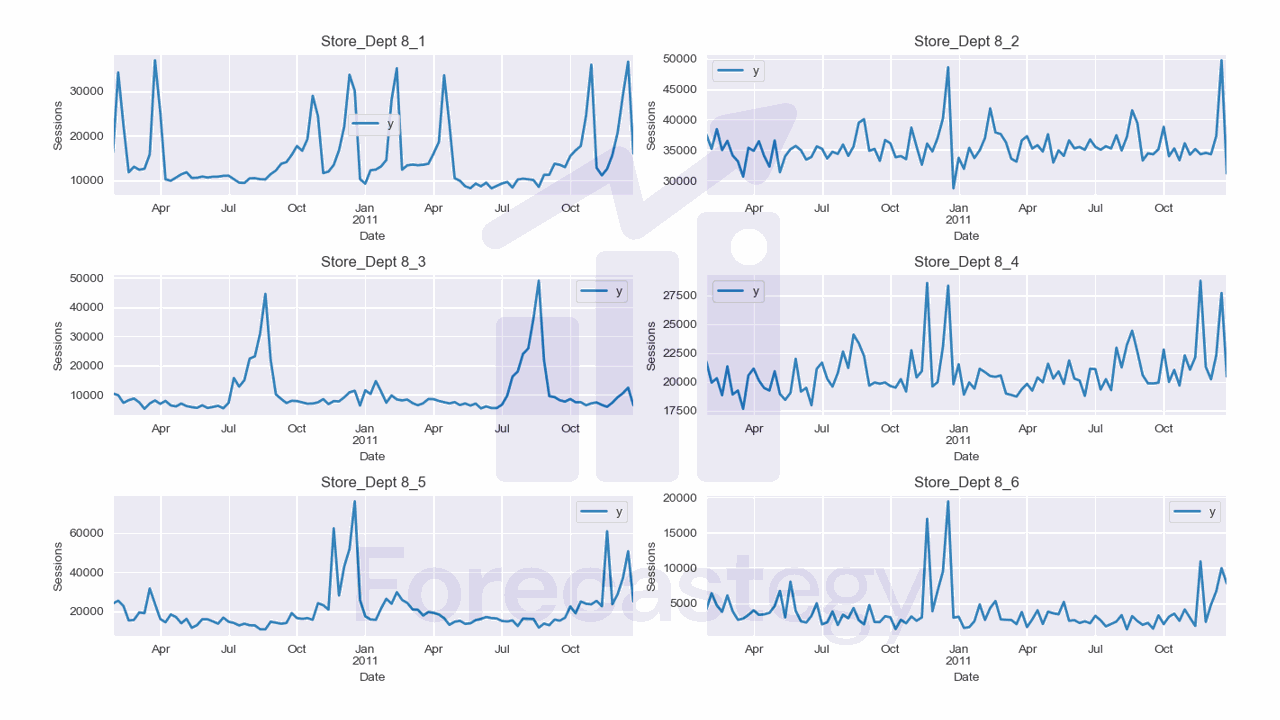
Let’s use the Walmart Sales Forecasting dataset from Kaggle.
This dataset contains the weekly sales, split by department, of 45 Walmart stores.
What matters most to us here is that it has additional information like temperature, fuel price, CPI, unemployment rate, store size, etc.
We’ll use this information to train a multivariate time series model to predict the weekly sales of specific departments in specific stores.
Let’s start by loading the data:
import pandas as pd
import numpy as np
from matplotlib import pyplot as plt
import os

data = pd.read_csv(os.path.join(path, 'train.csv'),
                   parse_dates=['Date'])
features = pd.read_csv(os.path.join(path, 'features.csv'),
                       parse_dates=['Date'])
stores = pd.read_csv(os.path.join(path, 'stores.csv'))
data is the main dataset.
| Store | Dept | Date | Weekly_Sales | IsHoliday |
|---|---|---|---|---|
| 1 | 1 | 2010-02-05 00:00:00 | 24924.5 | False |
| 1 | 1 | 2010-02-12 00:00:00 | 46039.5 | True |
| 1 | 1 | 2010-02-19 00:00:00 | 41595.6 | False |
| 1 | 1 | 2010-02-26 00:00:00 | 19403.5 | False |
| 1 | 1 | 2010-03-05 00:00:00 | 21827.9 | False |
It has the following columns:
Store: the store numberDept: the department numberDate: the date of the weekWeekly_Sales: the sales for the given department in the given store at the given dateIsHoliday: whether the week is a special holiday week
features contains additional variables with values for specific weeks.
| Store | Date | Temperature | Fuel_Price | MarkDown1 | MarkDown2 | MarkDown3 | MarkDown4 | MarkDown5 | CPI | Unemployment | IsHoliday |
|---|---|---|---|---|---|---|---|---|---|---|---|
| 1 | 2010-02-05 00:00:00 | 42.31 | 2.572 | nan | nan | nan | nan | nan | 211.096 | 8.106 | False |
| 1 | 2010-02-12 00:00:00 | 38.51 | 2.548 | nan | nan | nan | nan | nan | 211.242 | 8.106 | True |
| 1 | 2010-02-19 00:00:00 | 39.93 | 2.514 | nan | nan | nan | nan | nan | 211.289 | 8.106 | False |
| 1 | 2010-02-26 00:00:00 | 46.63 | 2.561 | nan | nan | nan | nan | nan | 211.32 | 8.106 | False |
| 1 | 2010-03-05 00:00:00 | 46.5 | 2.625 | nan | nan | nan | nan | nan | 211.35 | 8.106 | False |
The columns are:
Store: the store numberDate: the week when the data was recordedTemperature: average temperature in the regionFuel_Price: cost of fuel in the regionMarkDown1toMarkDown5: anonymized data related to promotional markdownsCPI: the consumer price indexUnemployment: the unemployment rateIsHoliday: whether the week is a special holiday week
We will remove the MarkDown columns, but use the rest of the features.
The stores dataset contains information about the store’s characteristics.
| Store | Type | Size |
|---|---|---|
| 1 | A | 151315 |
| 2 | A | 202307 |
| 3 | B | 37392 |
| 4 | A | 205863 |
| 5 | B | 34875 |
The columns are:
Store: the store numberType: the type of store (A, B or C)Size: the size of the store
Type is defined according to the size.
We merge everything into a single dataset:
data = pd.merge(data, features, on=['Store', 'Date', 'IsHoliday'], how='left')
data = pd.merge(data, stores, on=['Store'], how='left')
We need to do some preprocessing to make the data suitable for MLForecast.
First, we set the date of each week to be the Sunday of that week.
data['Date'] = data['Date'].dt.to_period('W-SAT').dt.start_time
I also removed the stores that didn’t have data for the whole period. You can use everything I teach here with time series that have different sizes, but for simplicity I’ll not do it here.
last_date_by_store = data.groupby('Store')['Date'].last()
stores_with_full_data = last_date_by_store[last_date_by_store == data['Date'].max()].index
data = data.loc[data['Store'].isin(stores_with_full_data)]
Let’s transform the categorical variables into one-hot encoded variables.
data['Type_A'] = (data['Type'] == 'A').astype(int)
data['Type_B'] = (data['Type'] == 'B').astype(int)
data['IsHoliday'] = data['IsHoliday'].astype(int)
I will use the very successful ensembles of tree-based models to predict the sales, so this transformation is not completely necessary, as they do well with ordinal encoding.
So I left Store and Dept as they are, but wanted to remind you of this option.
Now I will create a unique_id column joining Store and Dept, so that mlforecast knows they are different time series and can calculate the features accordingly.
data['unique_id'] = data['Store'].astype(str) + '_' + data['Dept'].astype(str)
data = data.drop(['MarkDown1', 'MarkDown2', 'MarkDown3',
                  'MarkDown4', 'MarkDown5', 'Type'], axis=1)
data = data.rename(columns={'Weekly_Sales': 'y', 'Date': 'ds'})
I also removed the MarkDown columns, as I said before. We don’t need Type anymore, as we have the one-hot encoded variables.
I renamed Weekly_Sales to y and Date to ds which is the format mlforecast expects for the target variable and the date.
Finally, let’s split the data into train and validation sets. We will use all data between 2010 and 2011 to train the model, and data from 2012 to validate it.
train = data.loc[data['ds'] < '2012-01-01']
valid = data.loc[data['ds'] >= '2012-01-01']
h = 4
h is the horizon, the number of steps we want to predict after the end of the training data, so I set it to 4 weeks.
The longer the horizon, the less accurate the predictions will be.
This is a sample of the data we will use to train the model:

Training A Multivariate Time Series Model In Python With MLForecast
Let’s see how we can engineer features and train an XGBoost and a Random Forest model easily with mlforecast.
from sklearn.ensemble import RandomForestRegressor
from sklearn.impute import SimpleImputer
from sklearn.pipeline import make_pipeline
from xgboost import XGBRegressor

from window_ops.rolling import rolling_mean, rolling_max, rolling_min

models = [make_pipeline(SimpleImputer(),
                        RandomForestRegressor(random_state=0, n_estimators=100)),
          XGBRegressor(random_state=0, n_estimators=100)]


model = MLForecast(models=models,
                   freq='W',
                   lags=[1,2,4],
                   lag_transforms={
                       1: [(rolling_mean, 4), (rolling_min, 4), (rolling_max, 4)], # aplicado a uma janela W a partir do registro Lag
                   },
                   date_features=['week', 'month'],
                   num_threads=6)
After importing the models we want, we need to put them in a list, and pass it to the MLForecast class.
Our models list contains a RandomForestRegressor and an XGBRegressor.
The RandomForestRegressor is inside a scikit-learn pipeline, so that we can use the SimpleImputer to fill any missing values in the data.
By default, SimpleImputer fills missing values with the mean of the column, but you can change that by passing the strategy parameter.
If you know your data doesn’t have missing values, you can remove the SimpleImputer from the pipeline.
You can use any scikit-learn model, or any other model that follows the same API. We could use LightGBM or CatBoost, for example.
You don’t need more than one model, but I wanted to show you that you can use more than one.
The MLForecast object will manage the transformation of the data, the training of the models, and the prediction of the target variable.
We pass the freq parameter to tell mlforecast that our data is weekly, and the lags parameter to tell it that we want to use the last 1, 2 and 4 weeks as features to predict the next week.
We also pass the lag_transforms parameter, which is a dictionary that maps the number of lags to a list of functions to apply to the lagged values.
The keys are the lags over which we want to apply the functions, and the values are lists of tuples, where the first element is the function to apply, and the second element is the number of weeks to apply it to (the window).
So in this case, we will apply the rolling_mean, rolling_min and rolling_max functions to the last 4 weeks of each lag.
To be very clear, if today is week 5, the function will be applied to the values of week 1, 2, 3 and 4.
I explained feature engineering for time series in detail in the article about multiple time series forecasting with scikit-learn.
The developers of mlforecast recommend we use the window_ops package or create our custom functions with numba.
date features is a list of the date components we want to use. These are features like the month, the week of the year, the day of the week (if it was a daily time series), etc.
Finally, num_threads is the number of threads to use when training the models in parallel. Setting it to the number of cores in your machine is a good idea.
Before we train the model, let’s create two lists with the names of the dynamic and static features.
dynamic_features = ['IsHoliday', 'Temperature', 'Fuel_Price', 'CPI', 'Unemployment']
static_features = ['Type_A', 'Type_B', 'Size', 'Store', 'Dept']
Dynamic features are the ones that change over time. You need to have these values for the future timestamps you want to predict.
Static features are the ones that don’t change over time. MLForecast will repeat the first value of each static feature for all the timestamps you want to predict.
Be careful with dynamic features!
In this case, the IsHoliday column is easy to know in advance, but the Temperature, Fuel_Price, CPI and Unemployment columns are not.
We would need to use estimates for these values when this model is deployed.
So, if you have this kind of feature, you can use the real historical values in your training set, but you should use estimates for the validation set and any future data.
If you use historical values for the validation set and future data, you will get an overoptimistic out-of-sample accuracy and have a bad surprise when you deploy your model.
As a rule of thumb, always ask the question: “Would I have this information if today was the last day of the training set? (the day you make the prediction)”.
With that in mind, let’s train the models.
model.fit(train, id_col='unique_id', time_col='ds', target_col='y', static_features=static_features)
We pass the training data, the name of the column with the unique identifier for each time series, the date, the target variable, and the list of static features.
If you have no static features, pass an empty list or MLForecast will consider that all your additional columns are static.
By default the forecast is generated in a recursive way, but we can also use the max_horizon parameter to generate the forecast with the direct method (one model for each step ahead);
model.fit(train, id_col='unique_id', time_col='ds', target_col='y', static_features=static_features, max_horizon=h)
After training the models, we can use it to predict the next h weeks.
p = model.predict(horizon=h, dynamic_dfs=[valid[['unique_id','ds']+dynamic_features]])
p = p.merge(valid[['unique_id', 'ds', 'y']], on=['unique_id', 'ds'], how='left')
We pass the horizon parameter to tell the model how many steps to predict after the end of the training data.
Be careful with the dates here if you have errors about missing values in your data.
This is why I had to set all the dates to the first Sunday of the week. The dates were not aligned between MLForecast and the validation data.
We also pass the dynamic_dfs parameter, which is a list of dataframes with the dynamic features for the validation set.
We need columns to join the dataframes, so we pass the unique_id and ds in the dynamic features dataframe.
Finally, we merge the predictions with the validation data to calculate the error metrics.
This is what p looks like at the end:
| unique_id | ds | Pipeline | XGBRegressor | y |
|---|---|---|---|---|
| 10_1 | 2012-01-01 00:00:00 | 48989.7 | 75332.5 | 28520.5 |
| 10_1 | 2012-01-08 00:00:00 | 46245.6 | 87932.9 | 30107.3 |
| 10_1 | 2012-01-15 00:00:00 | 46587.5 | 91423.3 | 31180.2 |
| 10_1 | 2012-01-22 00:00:00 | 54463.7 | 91988.7 | 32559.1 |
| 10_10 | 2012-01-01 00:00:00 | 50423.6 | 50885.7 | 37105.5 |
We can see the predictions for the Pipeline (Random Forest) and the XGBRegressor models, and the actual values.
To evaluate the model, I will use SMAPE, which helps us deal with zeros and negative values in the target variable.
Sometimes people use negative values in sales data to represent days when returns were higher than sales.
def smape(y_true, y_pred):
    return 100 * np.mean(np.abs(y_pred - y_true) / (np.abs(y_true) + np.abs(y_pred)))

print(f"SMAPE Random Forest Pipeline: {smape(p['y'], p['Pipeline'])}\nSMAPE XGBRegressor: {smape(p['y'], p['XGBRegressor'])}")
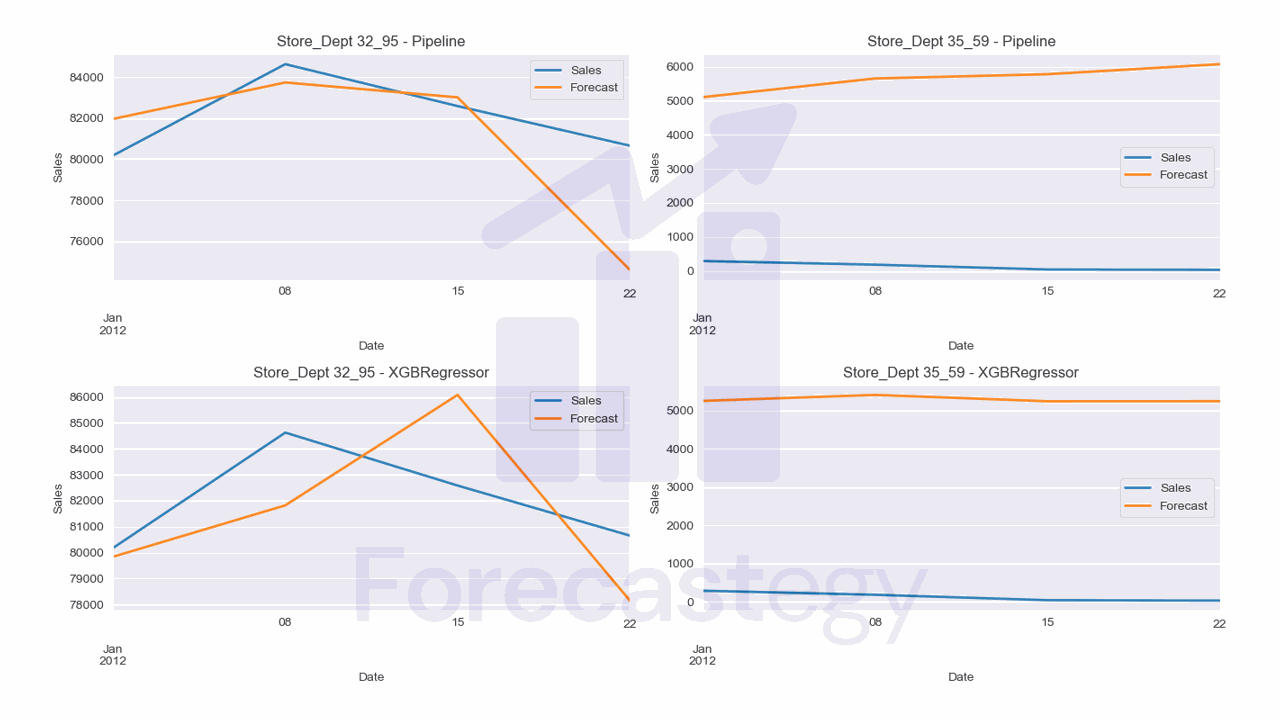
The Random Forest model got a 21.81% SMAPE, and the XGBoost model got a 23.05%.
I purposefully plotted the time series with the best (32_95) and worst (35_59) performance.
For the worst series, it seems the model doesn’t understand that the first weeks of January are usually low, and it predicts a high value.
If you want to improve the forecasts, I would first investigate the data and understand if there are any shocks or anomalies that could be affecting the model.
Another idea is to tune the hyperparameters of models.
Take a look at the feature importances too.
This model is heavily dependent on the lag 1 feature, as you can see in the feature importance plot for XGBRegressor.
pd.Series(model.models_['XGBRegressor'].feature_importances_, index=model.ts.features_order_).sort_values(ascending=False).plot.bar(title='Feature Importance XGBRegressor')
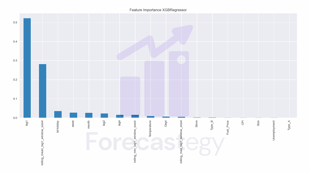
After the first week, lag 1 is the prediction for the previous week, so the model will accumulate errors as it goes. If the errors are large, the model will get worse and worse.
This is a pattern specific of this data, not the models or methods.
If you have a similar problem, I would try removing the lag 1 features and modeling with max_horizon to see if the direct method would work better.