
As a data scientist, tackling sales forecasting for multiple products is a tough job.
You know it’s essential for businesses, but dealing with different models, metrics, and complexities can be overwhelming.
You might be feeling the pressure to deliver accurate forecasts to drive better decision-making and wondering how to tackle this challenge effectively.
Don’t worry! I’m here to make this process easier and guide you through it.
In this tutorial, I’ll simplify sales forecasting by walking you through these key steps:
- Making a validation set for sales forecasting
- Creating and checking an initial baseline model
- Learning evaluation metrics like SMAPE, Pinball Loss, and Coverage Probability
- Trying techniques like ARIMA, Holt-Winters, and DeepAR (LSTM) models
- Fine-tuning DeepAR hyperparameters for the best results
By the end of this tutorial, you’ll be skilled in handling various sales forecasting models and techniques.
This will help you develop and refine forecasts for different products, leading to smarter decisions for your business.
Eager to level up your sales forecasting abilities? Let’s dive in!
This method is best-suited for products that have some sales history and sell almost every period.
Check our other tutorial for forecasting products with intermittent demand.
How To Transform Transactional Data For Sales Forecasting
To illustrate the importance of transforming transactional data into a sales forecasting-friendly format, let’s use an example from the retail industry.
Imagine a store selling a variety of products, like electronics, clothes, and toys.
Their raw transactional data would include details like product IDs, transaction timestamps, and quantities sold, but this information may be scattered across multiple tables or files.
By transforming this raw data into a more structured form, you can easily track the sales trends of different products over time.
Here we will work as if we were hired by a store that wants to forecast the sales performance of its top 100 most frequently sold products on a weekly basis.
You can expand this method to forecast the sales of more products or on a daily basis.
The final format we need the data to be in is the long format with each row containing: unique IDs for the products, a reference date and the quantity or dollar amount sold.
To show you how to do it, I found the Olist Brazilian E-Commerce Public Dataset on Kaggle, which contains real transactional data for a Brazilian e-commerce company from 2016 to 2018.
First, the code reads in two separate data files, one that contains order items and the other with order details.
Then, it merges the two data sources together using the 'order_id' as the common key to match the relevant information.
import os
import pandas as pd

order_items = pd.read_csv(os.path.join(path, 'olist_order_items_dataset.csv'))
orders = pd.read_csv(os.path.join(path, 'olist_orders_dataset.csv'))
orders = orders[['order_id', 'order_purchase_timestamp']]
data = pd.merge(order_items, orders, on='order_id')
This is what 'olist_order_items_dataset.csv' looks like:
| order_id | order_item_id | product_id | seller_id | shipping_limit_date | price | freight_value |
|---|---|---|---|---|---|---|
| 00010242fe8c5a6d1ba2dd792cb16214 | 1 | 4244733e06e7ecb4970a6e2683c13e61 | 48436dade18ac8b2bce089ec2a041202 | 2017-09-19 09:45:35 | 58.9 | 13.29 |
| 00018f77f2f0320c557190d7a144bdd3 | 1 | e5f2d52b802189ee658865ca93d83a8f | dd7ddc04e1b6c2c614352b383efe2d36 | 2017-05-03 11:05:13 | 239.9 | 19.93 |
| 000229ec398224ef6ca0657da4fc703e | 1 | c777355d18b72b67abbeef9df44fd0fd | 5b51032eddd242adc84c38acab88f23d | 2018-01-18 14:48:30 | 199 | 17.87 |
| 00024acbcdf0a6daa1e931b038114c75 | 1 | 7634da152a4610f1595efa32f14722fc | 9d7a1d34a5052409006425275ba1c2b4 | 2018-08-15 10:10:18 | 12.99 | 12.79 |
| 00042b26cf59d7ce69dfabb4e55b4fd9 | 1 | ac6c3623068f30de03045865e4e10089 | df560393f3a51e74553ab94004ba5c87 | 2017-02-13 13:57:51 | 199.9 | 18.14 |
And this is what selected columns of 'olist_orders_dataset.csv' looks like:
| order_id | order_purchase_timestamp |
|---|---|
| e481f51cbdc54678b7cc49136f2d6af7 | 2017-10-02 10:56:33 |
| 53cdb2fc8bc7dce0b6741e2150273451 | 2018-07-24 20:41:37 |
| 47770eb9100c2d0c44946d9cf07ec65d | 2018-08-08 08:38:49 |
| 949d5b44dbf5de918fe9c16f97b45f8a | 2017-11-18 19:28:06 |
| ad21c59c0840e6cb83a9ceb5573f8159 | 2018-02-13 21:18:39 |
After merging, this is the dataset we get:
| order_id | order_item_id | product_id | seller_id | shipping_limit_date | price | freight_value | order_purchase_timestamp |
|---|---|---|---|---|---|---|---|
| 00010242fe8c5a6d1ba2dd792cb16214 | 1 | 4244733e06e7ecb4970a6e2683c13e61 | 48436dade18ac8b2bce089ec2a041202 | 2017-09-19 09:45:35 | 58.9 | 13.29 | 2017-09-13 08:59:02 |
| 00018f77f2f0320c557190d7a144bdd3 | 1 | e5f2d52b802189ee658865ca93d83a8f | dd7ddc04e1b6c2c614352b383efe2d36 | 2017-05-03 11:05:13 | 239.9 | 19.93 | 2017-04-26 10:53:06 |
| 000229ec398224ef6ca0657da4fc703e | 1 | c777355d18b72b67abbeef9df44fd0fd | 5b51032eddd242adc84c38acab88f23d | 2018-01-18 14:48:30 | 199 | 17.87 | 2018-01-14 14:33:31 |
| 00024acbcdf0a6daa1e931b038114c75 | 1 | 7634da152a4610f1595efa32f14722fc | 9d7a1d34a5052409006425275ba1c2b4 | 2018-08-15 10:10:18 | 12.99 | 12.79 | 2018-08-08 10:00:35 |
| 00042b26cf59d7ce69dfabb4e55b4fd9 | 1 | ac6c3623068f30de03045865e4e10089 | df560393f3a51e74553ab94004ba5c87 | 2017-02-13 13:57:51 | 199.9 | 18.14 | 2017-02-04 13:57:51 |
Now we have information about when the order was made and we can count how much of each product was sold each period.
The data is already in the long format, where each row represents a single observation, and each column represents a different attribute of that observation.
data_long = data[['product_id', 'order_purchase_timestamp', 'order_item_id']].copy()

data_long['order_purchase_timestamp'] = pd.to_datetime(data_long['order_purchase_timestamp']).dt.normalize()
data_long = data_long[data_long['order_purchase_timestamp'] >= '2017-01-01']
data_long['week_start_date'] = (data_long['order_purchase_timestamp'] + pd.Timedelta(days=1)).apply(lambda x: x - pd.offsets.Week(weekday=6))
In this case, each observation is a product sold, and the attributes are the product’s ID, the date it was sold, and the number of units sold.
The data is filtered to only include orders made on or after '2017-01-01' and we create a new column 'week_start_date' that will be our reference period to aggregate the data.
The purpose of this particular code segment is to assign a consistent week_start_date to every transaction in the dataset.
Be very careful when dealing with dates, because it’s very easy to get confused about the exact date a period starts or ends.
In this case, I had to experiment with multiple transformations until I found one that worked.
Here’s a breakdown of the line that creates the 'week_start_date' column:
data_long['order_purchase_timestamp']contains the purchase dates for each transaction.pd.Timedelta(days=1)is used to add one day to the purchase date, which helps account for transactions occurring on the starting weekday (Sunday).(data_long['order_purchase_timestamp'] + pd.Timedelta(days=1)).apply(lambda x: x - pd.offsets.Week(weekday=6))calculates theweek_start_datefor each transaction by rolling back the date to the most recent Sunday.
Next, the data is grouped by 'product_id' and 'week_start_date', counting the number of units sold each week for each product.
This new aggregated table is then renamed from 'order_item_id' to 'quantity_sold' to more accurately reflect its contents.
To focus on the top 100 best-selling products, the data is further filtered for these specific items.
data_grouped = data_long.groupby(['product_id', 'week_start_date'])['order_item_id'].sum().reset_index()

data_grouped = data_grouped.rename(columns={'order_item_id': 'quantity_sold'})

top100 = data_grouped['product_id'].value_counts().head(100).index
data_grouped = data_grouped[data_grouped['product_id'].isin(top100)]
| product_id | week_start_date | quantity_sold |
|---|---|---|
| 0152f69b6cf919bcdaf117aa8c43e5a2 | 2017-02-19 00:00:00 | 1 |
| 0152f69b6cf919bcdaf117aa8c43e5a2 | 2017-03-05 00:00:00 | 4 |
| 0152f69b6cf919bcdaf117aa8c43e5a2 | 2017-03-12 00:00:00 | 6 |
| 0152f69b6cf919bcdaf117aa8c43e5a2 | 2017-03-19 00:00:00 | 6 |
| 0152f69b6cf919bcdaf117aa8c43e5a2 | 2017-03-26 00:00:00 | 4 |
All the products are “stacked” on top of each other in the same DataFrame.
One problem we still have is that not every product has been sold every week, so there are missing values in the data.
We want each product to have a value for every week, even if it’s zero.
So we use the pivot method to transform the data into wide format, where each row represents a single product, and each column represents a different week.
Then, after filling in the missing values with zeros, we use the stack method to transform the data back into long format.
data_pivoted = data_grouped.pivot(index='product_id', columns='week_start_date', values='quantity_sold').fillna(0)

data_long = data_pivoted.stack().reset_index()
data_long = data_long.rename(columns={'level_1': 'week_start_date', 0: 'quantity_sold'})
The final format is the same as the last table above, but now we have a value for every product for every week.
If your data contains missing data because of the way it was collected instead of simple sparsity (like in this case), you should be careful about filling in the missing values.
We can verify that all products have the same number of observations by ensuring that the standard deviation of the row count per product is zero.
assert data_long.groupby('product_id').size().describe()['std'] == 0
Finally, we rename the columns to match the requirements of the libraries we’ll be testing for forecasting.
data_long = data_long.rename(columns={'week_start_date': 'ds', 'quantity_sold': 'y', 'product_id': 'unique_id'})
How To Create a Validation Set For Sales Forecasting
Now that we have transformed our transactional data into a forecasting-friendly format, the next crucial step is to create a validation set.
A validation set is used to evaluate the performance of the model before we use it for future sales predictions.
To create a validation set, we’ll split our data into a training dataset and a validation dataset.
We could have a test dataset as well but, in my experience, you can make a lot of mistakes that render your test set unreliable, so I take production data as the real test set.
Here’s the code to split the data:
train = data_long[data_long['ds'] < '2018-01-01']
valid = data_long[(data_long['ds'] >= '2018-01-01') & (data_long['ds'] < '2018-03-01')]
h = valid['ds'].nunique()
print('h =', h)

print('train:', train)
print('valid:', valid)
We split the data into three parts:
- Training: This dataset includes all records before ‘2018-01-01’. We will use it to train our forecasting models.
- Validation: This dataset includes records between ‘2018-01-01’ and ‘2018-03-01’. We will use this data to validate our model’s performance and fine-tune its parameters.
The variable h is used to represent the forecasting horizon.
The forecasting horizon is the number of time periods into the future that we want to forecast.
In this case, h represents the number of weeks in our validation set, which we will use to forecast sales.
Now, with the training and validation sets, we can proceed to fit our sales forecasting models, evaluate their performances, and make predictions.
How to Build an Initial Sales Forecasting Baseline Model
Establishing a baseline is an essential step in the sales forecasting process.
Creating a simple baseline model helps you understand the sales forecasting problem better and provides a base performance level that more complex models should aim to surpass.
In other words, deploying complex models isn’t worth it if they can’t outperform a simple baseline.
In this section, we will use a selection of basic models to create a foundation for our sales forecasting.
Importing Libraries and Creating Baseline Models
First, we’ll import the necessary libraries and establish a variety of basic models.
These include:
Naive: A naive model that assumes sales will be the same as the most recent observation.SeasonalNaive: A model that takes seasonality into account and repeats the sales pattern from the previous season.WindowAverage: A moving average model that calculates the average sales over a specified window of previous observations.SeasonalWindowAverage: A model that captures both seasonality and a moving average by combining the seasonal naive and window average approaches.
In our case, a season is (arbitrarily) defined as 4 weeks. We expect that the sales pattern for a given product will be similar every 4 weeks.
It makes sense if you think about salary payments and credit card bills due dates.
The right seasonal length will depend on the data and the problem you’re trying to solve.
Talk with domain experts to determine the right season length for your problem.
We will use the StatsForecast library to create these models.
You can easily install it using pip:
pip install statsforecast
Or conda:
conda install -c nixtla statsforecast
Here’s the code to import the libraries and set up these baseline models:
from statsforecast import StatsForecast
from statsforecast.models import Naive, SeasonalNaive, WindowAverage, SeasonalWindowAverage

model = StatsForecast(models=[Naive(),
                              SeasonalNaive(season_length=4),
                              WindowAverage(window_size=4),
                              SeasonalWindowAverage(window_size=2, season_length=4)],
                      freq='W', n_jobs=-1)
Fitting the Baseline Models
With the baseline models set up, we’ll now fit them using our training dataset:
model.fit(train)
Generating Forecasts and Evaluating Performance
After fitting the models, we can generate forecasts for the validation dataset.
Remember that, in this example, we use a forecasting horizon (h) equal to the number of unique dates in the validation dataset.
I used 9 weeks, but you can change this value to any number of weeks you want.
p = model.forecast(h=h, level=[90])
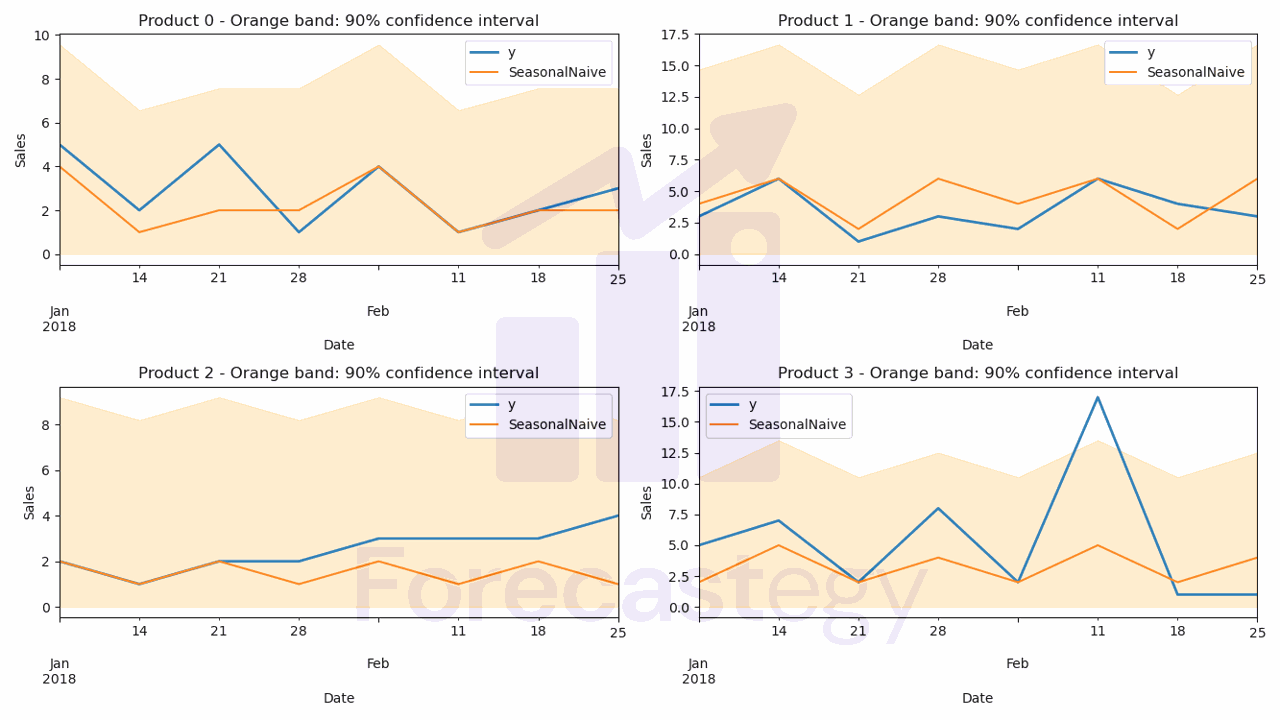
level is a parameter that controls the prediction interval.
Point forecasts provide a single estimate for the future, while prediction intervals show a range where the actual value might be.
Working with non-technical stakeholders, these intervals help create realistic expectations about the model’s performance, which leads to improved planning and decision-making.
Again, you can change this value to any number that is appropriate for your problem.
This is what the p dataframe looks like:
| ds | Naive | Naive-lo-90 | Naive-hi-90 | SeasonalNaive | SeasonalNaive-lo-90 | SeasonalNaive-hi-90 | WindowAverage | SeasWA |
|---|---|---|---|---|---|---|---|---|
| 2018-01-07 00:00:00 | 1 | -0.644854 | 2.64485 | 0 | -4.45428 | 4.45428 | 0.5 | 0 |
| 2018-01-14 00:00:00 | 1 | -1.32617 | 3.32617 | 1 | -3.45428 | 5.45428 | 0.5 | 0.5 |
| 2018-01-21 00:00:00 | 1 | -1.84897 | 3.84897 | 0 | -4.45428 | 4.45428 | 0.5 | 0 |
| 2018-01-28 00:00:00 | 1 | -2.28971 | 4.28971 | 1 | -3.45428 | 5.45428 | 0.5 | 0.5 |
| 2018-02-04 00:00:00 | 1 | -2.678 | 4.678 | 0 | -4.45428 | 4.45428 | 0.5 | 0 |
It has a column for each model, including the point forecast and the prediction interval bounds we specified for the models that support it.
In our case, negative values make no sense, so we’ll replace them with zeros:
cols = ['Naive', 'Naive-lo-90', 'Naive-hi-90', 'SeasonalNaive',
       'SeasonalNaive-lo-90', 'SeasonalNaive-hi-90', 'WindowAverage',
       'SeasWA']
p.loc[:, cols] = p.loc[:, cols].clip(0)
Finally, we merge the forecasts with the actual sales from the validation dataset to evaluate the models’ performance.
p = p.reset_index().merge(valid, on=['ds', 'unique_id'], how='left')
| unique_id | ds | Naive | Naive-lo-90 | Naive-hi-90 | SeasonalNaive | SeasonalNaive-lo-90 | SeasonalNaive-hi-90 | WindowAverage | SeasWA | y |
|---|---|---|---|---|---|---|---|---|---|---|
| 0152f69b6cf919bcdaf117aa8c43e5a2 | 2018-01-07 00:00:00 | 1 | 0 | 2.64485 | 0 | 0 | 4.45428 | 0.5 | 0 | 2 |
| 0152f69b6cf919bcdaf117aa8c43e5a2 | 2018-01-14 00:00:00 | 1 | 0 | 3.32617 | 1 | 0 | 5.45428 | 0.5 | 0.5 | 1 |
| 0152f69b6cf919bcdaf117aa8c43e5a2 | 2018-01-21 00:00:00 | 1 | 0 | 3.84897 | 0 | 0 | 4.45428 | 0.5 | 0 | 1 |
| 0152f69b6cf919bcdaf117aa8c43e5a2 | 2018-01-28 00:00:00 | 1 | 0 | 4.28971 | 1 | 0 | 5.45428 | 0.5 | 0.5 | 0 |
| 0152f69b6cf919bcdaf117aa8c43e5a2 | 2018-02-04 00:00:00 | 1 | 0 | 4.678 | 0 | 0 | 4.45428 | 0.5 | 0 | 0 |
Now that we have our baseline models in place, we can compare their performance with more complex models.
A well-performing complex model should outperform these baseline models, justifying any additional computational complexity and efforts needed in model development and deployment.
How To Evaluate a Sales Forecasting Model
To assess the performance of a sales forecasting model, we need to use multiple evaluation metrics.
In this section, we will focus on three key metrics: the Symmetric Mean Absolute Percentage Error (SMAPE) for point forecasts, the pinball loss for quantile metrics, and the coverage probability.
Symmetric Mean Absolute Percentage Error (SMAPE)
SMAPE is a scale-independent measure of accuracy that considers both underestimation and overestimation errors.
It’s particularly useful for sales forecasting because it allows for a fair comparison of forecasts even if sales values vary widely across products or time and can handle zero values in the true sales data.
Still, when evaluating sales forecasting models using SMAPE, it’s essential to be cautious about interpreting the percentage errors for products with low sales volumes.
For example, when comparing a 50% error in a product that sells 2 units versus a 50% error in a product that sells 100 units, the error in absolute terms is quite different.
In the first case, the 50% error translates to an error of only 1 unit, while in the second case, it corresponds to an error of 50 units.
In practical terms, the impact of the two errors on inventory management or revenue is very different.
Make sure to consider the practical implications of the errors in terms of units or revenue.
Here’s how we calculate SMAPE for the Naive model:
import numpy as np

def smape_loss(y_true, y_pred):
    return 100 * np.mean(np.abs(y_true - y_pred) / (np.abs(y_true) + np.abs(y_pred)))

print(smape_loss(p['y'], p['Naive']))
Pinball Loss
Pinball loss is a specialized metric for evaluating the accuracy of quantile forecasts, which estimate specific percentile values of the future sales distribution rather than just a single point.
For example, when predicting the 95th percentile sales volume of a product, pinball loss assesses how well the model estimates that specific quantile.
An accurate 95th percentile forecast means you can better estimate the upper range of potential sales outcomes, which allows you to avoid overstocking and reduce the risk of stockouts.
A lower pinball loss indicates a more accurate prediction, while a higher value suggests less precision.
To calculate the pinball loss, we use the mean_pinball_loss function from the sklearn.metrics module:
from sklearn.metrics import mean_pinball_loss

print(mean_pinball_loss(p['y'], p['Naive-lo-90'], alpha=0.05), mean_pinball_loss(p['y'], p['Naive-hi-90'], alpha=0.95))
As level is set to cover 90% of the distribution, the alpha value for the lower quantile is 0.05, and the alpha value for the upper quantile is 0.95.
It’s very easy to confuse the alpha value with the level.
Coverage Probability
Coverage probability measures how often the actual sales values lie within the prediction intervals.
A high coverage probability indicates that the true sales values often lie within the predicted range, giving you confidence in your model’s ability to provide reliable estimates of future sales.
When measuring 90% prediction intervals, you are aiming for a model that provides a range within which the true sales values should fall 90% of the time.
If your calculated coverage probability significantly deviates from the target 90%, it could indicate that your model’s prediction intervals may not be reliable.
For example, if your coverage probability is only 75%, it means that the true sales values fall within the prediction intervals only 75% of the time, which is lower than the desired 90%.
Then you need to go back and investigate why your model is not providing accurate prediction intervals.
Here’s how to calculate the coverage probability:
def coverage_prob(y_true, y_lo, y_hi):
    return np.mean((y_lo <= y_true) & (y_true <= y_hi))

print(coverage_prob(p['y'], p['Naive-lo-90'], p['Naive-hi-90']))
Now that you have the three metrics and understand their definitions, you can use them to compare the performance of the baseline models with the more complex models considering multiple aspects.
Some models might improve all three metrics, while others might improve only one or two.
For example, the model with lowest SMAPE have accurate point forecasts, but low Coverage Probability may suggest you should put effort into improving the prediction intervals.
Now let’s move on to more advanced forecasting techniques using ARIMA and Holt-Winters models.
How To Forecast Sales With ARIMA and Holt-Winters
First, let’s import the necessary libraries and set up our models.
We’re going to use the StatsForecast library again.
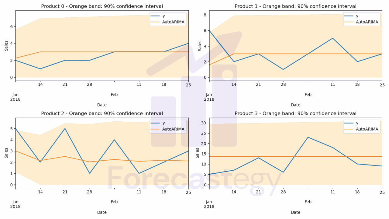
In this case, we’ll use two objects: AutoARIMA and HoltWinters.
ARIMA (Autoregressive Integrated Moving Average) is a linear model that combines three key components: autoregression (AR), differencing (I), and moving average (MA).
The AR component is based on the relationship between a current observation and a certain number of lagged observations (past values).
The I component helps make the time series stationary by subtracting the previous observation from the current one.
The MA component considers the relationship between a current observation and a residual error from a moving average model applied to lagged observations.
ARIMA models can capture complex patterns, like trends and seasonality, in the data.
They’re particularly useful for univariate time series data without external factors affecting the observations.
Holt-Winters is a model specifically designed for time series data that exhibits both trend and seasonality.
It’s an extension of the Simple Exponential Smoothing (SES) model, which weighs past observations with a decreasing exponential scale.
Holt-Winters improves upon SES by accounting for trends (using Holt’s linear trend method) and seasonal components (using a seasonal smoothing factor).
I chose to use ARIMA and Holt-Winters in this tutorial because they’re well-established methods with a solid track record in the field of time series forecasting.
They can handle various data patterns and often produce reliable forecasts for multiple products, making them a good fit for our e-commerce sales prediction problem.
Additionally, both models can be easily implemented and fine-tuned using Python libraries, which makes them practical for real-world applications.
from statsforecast import StatsForecast
from statsforecast.models import AutoARIMA, HoltWinters

model = StatsForecast(models=[AutoARIMA(season_length=4),
                              HoltWinters(season_length=4, error_type='A')],
                      freq='W', n_jobs=-1)
StatsForecast will apply an internal optimization process to find the best parameters for each model and product.
These models are local, not global, meaning that each product will have its own separate model, which is different than the global models we will see later.
Non-global models offer flexibility and easier interpretation at the cost of scalability and leveraging shared information across products.
There is no way to know if a global or local model will perform better before testing, so it’s best to try both and see which one works best for your data.
That said, these simpler, local models, tend to work better when we are doing long-term forecasts, as we usually have a smaller number of data points to train the model.
Now that we have our models set up, we need to fit them to our training data and get the forecasts.
As we are using the same library as for the naive baselines, the process is very similar:
model.fit(train)

p = model.forecast(h=h, level=[90])

cols = p.columns[1:]
p.loc[:, cols] = p.loc[:, cols].clip(0)
p = p.reset_index().merge(valid, on=['ds', 'unique_id'], how='left')
To evaluate these models, we’ll use the same metrics as before: SMAPE, Pinball Loss, and Coverage Probability.
print(smape_loss(p['y'], p['AutoARIMA']))
print(mean_pinball_loss(p['y'], p['AutoARIMA-lo-90'], alpha=0.1), mean_pinball_loss(p['y'], p['AutoARIMA-hi-90'], alpha=0.9))
print(coverage_prob(p['y'], p['AutoARIMA-lo-90'], p['AutoARIMA-hi-90']))
Now, how do you compare these metrics to the ones from the naive baselines?
In this dataset, the Naive model has about 63% SMAPE, while the ARIMA model has about 61% SMAPE.
Point for ARIMA.
But when it comes to Coverage Probability, the Naive model has 86%, while the ARIMA model has only 77%.
Point for Naive.
So if you had to pick between only these two, you would need to decide which metric is more important for your business or keep looking for a better model.
How To Forecast Sales With DeepAR (LSTM) And External Features
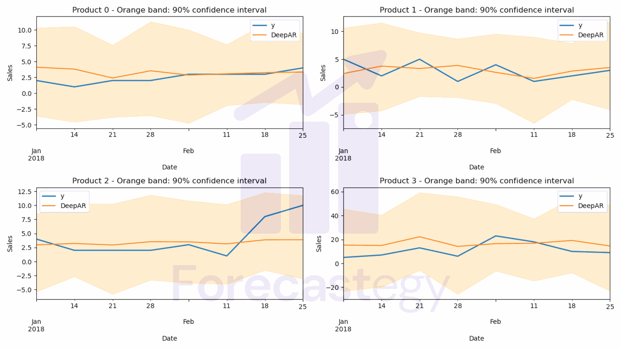
Now, let’s explore a more advanced technique for sales forecasting: DeepAR.
This is a global model that uses Long Short-Term Memory (LSTM), a type of recurrent neural network, to predict future values based on the past values of multiple time series.
DeepAR can capture complex patterns and dependencies among different products, making it suitable for our e-commerce sales prediction problem.
Originally it was developed for univariate time series, but GluonTS, the library we’ll use to implement DeepAR, has extended it to multivariate time series.
First I will add a static feature to the dataset.
products = pd.read_csv(os.path.join(path, 'olist_products_dataset.csv')).rename(columns={'product_id': 'unique_id'})
data_long_w_external = data_long.merge(products[['unique_id', 'product_category_name']], on='unique_id', how='left')
data_long_w_external['product_category_name'] = data_long_w_external['product_category_name'].astype('category')
cat_cardinality = data_long_w_external['product_category_name'].nunique()
This is what 'olist_products_dataset.csv' looks like:
| unique_id | product_category_name | product_name_lenght | product_description_lenght | product_photos_qty | product_weight_g | product_length_cm | product_height_cm | product_width_cm |
|---|---|---|---|---|---|---|---|---|
| 1e9e8ef04dbcff4541ed26657ea517e5 | perfumaria | 40 | 287 | 1 | 225 | 16 | 10 | 14 |
| 3aa071139cb16b67ca9e5dea641aaa2f | artes | 44 | 276 | 1 | 1000 | 30 | 18 | 20 |
| 96bd76ec8810374ed1b65e291975717f | esporte_lazer | 46 | 250 | 1 | 154 | 18 | 9 | 15 |
| cef67bcfe19066a932b7673e239eb23d | bebes | 27 | 261 | 1 | 371 | 26 | 4 | 26 |
| 9dc1a7de274444849c219cff195d0b71 | utilidades_domesticas | 37 | 402 | 4 | 625 | 20 | 17 | 13 |
In this code snippet, we’re preparing the dataset to include an external feature, product_category_name.
We could use all others, but for simplicity, we’ll use only this one.
Adding external features to the dataset is optional, but it can improve the model’s performance by providing additional information about the time series.
By including the category of each product, we hope that the model will be able to learn that some categories have different sales patterns than others, like seasonality.
The products dataset is read from a CSV file, and the column containing product IDs is renamed to unique_id for consistency.
The original dataset (data_long) is merged with the products dataset, essentially adding a new column - product_category_name - to the existing dataset.
This operation is performed using the unique_id as the common key between both datasets.
The product_category_name column is converted to a categorical data type.
This is an important step because categorical features are handled differently from numerical features in machine learning models.
The cardinality of the product_category_name column is calculated, which is the number of unique product categories present in the dataset.
This information will be used later when setting up the DeepAR model.
As we are passing it as a static categorical feature, DeepAR will automatically add this to the series when we make forecasts.
It’s possible to add dynamic features as well, like the periods in the historical data and forecast horizon when the product was on sale, or the price.
The downside is that you must have this information for the entire forecast horizon at the time of making the forecast, which is not always possible.
If you don’t have GluonTS installed, you can install it by following the instructions here.
We will use the PyTorch backend.
Let’s import the necessary libraries and prepare our dataset.
from gluonts.dataset.pandas import PandasDataset

train_ds = PandasDataset.from_long_dataframe(train, target='y', item_id='unique_id',
                                       timestamp='ds', freq='W', static_feature_columns=['product_category_name'])
Here, we’re creating a PandasDataset object from our training data using the from_long_dataframe method.
This method transforms the long format train DataFrame into a format suitable for use with the gluonts library.
The method takes the following attributes:
train: The input training DataFrame.target: The name of the target variable in the DataFrame (‘y’ in this case, which represents sales).item_id: The column that identifies different time series within the DataFrame (‘unique_id’ in this case, which represents individual products).timestamp: The column containing the time information (‘ds’ in this case, which represents the date).freq: The frequency of the time series data (‘W’ in this case, denoting weekly data).static_feature_columns: A list of column names that contain static (non-time-varying) features. In this case, we’re including the ‘product_category_name’ column as a static feature to improve our model’s performance.
Now, let’s set up the DeepAR model using the gluonts.torch.model.deepar module.
There are many parameters we can tune, but for now we’ll specify the number of layers, the static features, and the training parameters for the optimizer.
from gluonts.torch.model.deepar import DeepAREstimator

estimator = DeepAREstimator(freq='W', prediction_length=h, num_layers=1, num_feat_static_cat=1,
                            cardinality=[cat_cardinality],
                            trainer_kwargs={'accelerator': 'gpu','max_epochs':1})
In this code snippet, we’re setting up the DeepAR model using the DeepAREstimator class.
The model’s arguments are defined as follows:
freq: The frequency of the time series data (‘W’ for weekly data).prediction_length: The number of time steps to predict into the future (denoted ashhere).num_layers: The number of layers in the LSTM neural network (set to 1 in this case).num_feat_static_cat: The number of static categorical features we’re including in the model (1 in this case, representing the ‘product_category_name’ feature).cardinality: A list containing the cardinality (number of distinct categories) of each static categorical feature. In our case, we provide[cat_cardinality], a list with a single element, which is the number of unique product categories in our dataset.trainer_kwargs: A dictionary containing additional arguments for the model’s optimizer. In this case, we specify to use a GPU accelerator for faster training and set the maximum number of training epochs to 1. Training epochs refer to the number of times the model will see the entire training dataset during training.
Next, we’ll train the model using our prepared dataset with the train method.
predictor = estimator.train(train_ds)
Once the model is trained, we can use the predict method to generate forecasts for each product in our dataset.
The predict method returns a generator object, which we can convert to a list and then to a DataFrame.
DeepAR estimates the parameters of a distribution for each time step in the forecast horizon, so each element in the list contains samples from the fitted distribution as forecasts.
def make_df_preds(predictor, dataset):
    pred = list(predictor.predict(dataset))
    # gluonts.model.forecast.SampleForecast(info=None, item_id='0152f69b6cf919bcdaf117aa8c43e5a2', samples=array([[ 1.53543979e-01,  4.16583046e-02,  2.44526476e-01...]], dtype=float32), start_date=Period('2018-01-01/2018-01-07', 'W-SUN'))
    all_preds = list()
    for item in pred:
        unique_id = item.item_id
        p = item.samples.mean(axis=0)
        plo = np.percentile(item.samples, 5, axis=0)
        phi = np.percentile(item.samples, 95, axis=0)
        dates = pd.date_range(start=item.start_date.to_timestamp(), periods=len(p), freq='W')
        category_pred = pd.DataFrame({'ds': dates, 'unique_id': unique_id, 'pred': p, 'plo': plo, 'phi': phi})
        all_preds += [category_pred]
    all_preds = pd.concat(all_preds, ignore_index=True)
    return all_preds

all_preds = make_df_preds(predictor, train_ds)
all_preds = all_preds.merge(valid[['unique_id', 'ds', 'y']], on=['unique_id', 'ds'], how='left')
In this code snippet, we define a function called make_df_preds that generates forecasts using the trained DeepAR model and formats the results into a DataFrame.
The function takes two arguments:
predictor: The trained DeepAR model.dataset: The dataset for which we want to generate forecasts.
Inside the function, we perform the following steps:
-
Call the
predictmethod of thepredictorto generate forecasts for each time series in the dataset. The results are stored in a list calledpred. -
Initialize an empty list named
all_predsto store the formatted forecasts for each time series. -
Iterate through the items in
pred. For each item, we:- Extract the unique ID (product ID) and store it in
unique_id. - Compute the mean forecast across all generated samples and store it in
p. - Calculate the 5th and 95th percentiles of the forecast samples, and store them in
ploandphi, respectively. These values represent the lower and upper bounds of the 90% prediction interval. - Create a date range starting from the first date in the forecast and continuing for the desired prediction length (
len(p)), using a weekly frequency (‘W’). - Create a DataFrame called
category_predthat contains the date, unique ID, mean forecast, and the 10th and 90th percentiles for each time step. - Append
category_predto theall_predslist.
- Extract the unique ID (product ID) and store it in
-
Concatenate all the DataFrames stored in
all_preds, and reset the index to create a unified DataFrame containing all the forecasts.
After defining the make_df_preds function, we use it to generate forecasts for our training dataset (train_ds) and store the results in the all_preds DataFrame.
Why train_ds instead of valid_ds?
DeepAR will use this data as context and generate forecasts for the immediate future (the next h weeks) from the last date in the training data.
Finally, we merge the all_preds DataFrame with the validation data using common columns (unique_id and ds) to facilitate the comparison and evaluation of the forecasts.
Now, we can evaluate the DeepAR model using the same metrics as before: SMAPE, Pinball Loss, and Coverage Probability.
How To Tune DeepAR Hyperparameters
It’s unlikely that we’ll get the best possible results with the default hyperparameters, so let’s try to improve our model’s performance by tuning the hyperparameters with Optuna.
Optuna is a powerful hyperparameter optimization library that helps us find the best combination of hyperparameters for our model.
Installing it is very simple with pip:
pip install optuna
First, we need to define the objective function that Optuna will use to evaluate different sets of hyperparameters.
import optuna

def objective(trial):
    num_layers = trial.suggest_int('num_layers', 1, 4)
    context_length = trial.suggest_int('context_length', 4, 52)
    hidden_size = trial.suggest_categorical('hidden_size', [8, 16, 32, 64, 128, 256])
    dropout_rate = trial.suggest_float('dropout_rate', 0.0, 0.95)
    lr = trial.suggest_float('lr', 1e-5, 1e-1, log=True)
    batch_size = 256

    estimator = DeepAREstimator(freq='W', prediction_length=h, num_feat_static_cat=1,
                            cardinality=[cat_cardinality], num_layers=num_layers,
                            context_length=context_length, hidden_size=hidden_size,
                            dropout_rate=dropout_rate, batch_size=batch_size, lr=lr,
                            trainer_kwargs={'accelerator': 'gpu','max_epochs':10})
    predictor = estimator.train(train_ds)

    df_preds = make_df_preds(predictor, train_ds)
    df_preds = df_preds.merge(valid, on=['ds', 'unique_id'], how='left')

    return coverage_prob(df_preds['y'], df_preds['plo'], df_preds['phi'])
Inside the objective function, we create a DeepAR model with the given hyperparameters, train it using our training dataset, and generate forecasts like before.
Then, the forecasts are evaluated using the Coverage Probability metric, which is returned as the optimization target.
Here is a brief explanation of each hyperparameter and the ranges we’re exploring with Optuna:
-
num_layers: The number of layers in the LSTM neural network. The range we’re exploring is between 1 and 4 layers. More layers can capture complex patterns but may also add complexity and risk overfitting. -
context_length: The number of past time steps the model should consider when making a prediction. We’re trying values between 4 and 52, which represent 1 month to 1 year of historical data. A larger context length enables the model to learn from long-term trends but may increase computational complexity. -
hidden_size: The number of hidden units (neurons) in each LSTM layer. We’re testing a range of values: [8, 16, 32, 64, 128, 256]. Larger hidden sizes can make the model more expressive but may also increase computational cost and risk overfitting. GPUs tend to be faster with multiples of 2. -
dropout_rate: The dropout rate applied to the LSTM layers to prevent overfitting. We’re looking for values between 0.0 and 0.95. Higher dropout rates increase the regularization strength, but if it’s too high, the model may underfit the data. -
lr: The learning rate for the model’s optimizer. We’re trying values between 1e-5 and 1e-1 on a logarithmic scale. The learning rate controls how quickly the model updates its weights during training, and choosing an appropriate value is crucial for convergence and model performance. -
batch_size: The number of samples used for each update of the model’s weights during training. In this case, we set it to 256. Larger batch sizes can lead to faster training but may also require more memory and may result in less accurate estimation of the gradients.
After defining the objective function, we create an Optuna study with the direction set to 'maximize' since we want to maximize the Coverage Probability.
study = optuna.create_study(direction='maximize')
study.optimize(objective, n_trials=20)
We then call the optimize method and pass the objective function and the number of trials (20 in this case) as arguments.
Optuna will perform 20 optimization trials, searching for the best hyperparameter values to maximize our selected metric.
In practice, 20 to 30 trials are usually enough to find a good set of hyperparameters.
We can save all models during the optimization process or get the best set of hyperparameters at the end of the trials.
Then we retrain it and make the final forecasts or save the model for later use.