In today’s article, we’re going to explore the ins and outs of training a Holt-Winters model for forecasting multiple time series in Python.
Holt-Winters is a very popular forecasting algorithm that can capture seasonality and trends in time series data through exponential smoothing.
I’ll use StatsForecast, a scalable and easy-to-use Python library that can help you train a Holt-Winters model quickly and efficiently.
You don’t need to be a programming wizard to get started with this library, and it can save you hours of coding time.
Additionally, I’ll show you how to train a single time-series Holt-Winters model with StatsModels, a popular Python library for time series analysis.
Let’s begin!
How To Install StatsForecast
StatsForecast is available on PyPI, so you can install it with pip:
pip install statsforecast
Or with conda:
conda install -c conda-forge statsforecast
How To Prepare The Data For Holt-Winters
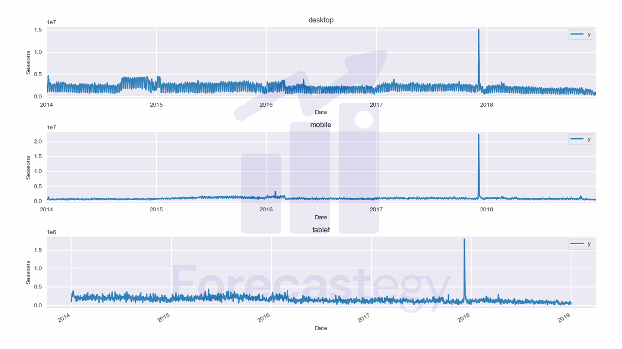
We will use data from the City of Los Angeles website traffic dataset on Kaggle.
This dataset contains the number of user sessions for the City of Los Angeles website for each day from 2014 to 2019.
Sessions are periods of time when a user is actively using the website.
Usually they are measured by looking at user activity and have a timeout after 30 minutes since the last user action.
For example, right now you are in a session on my website. If you leave the page and come back after 2 hours, you will be in a new session.
Let’s load the data and take a look at it:
import pandas as pd
import numpy as np
from matplotlib import pyplot as plt
import os

data = pd.read_csv(os.path.join(path, 'lacity.org-website-traffic.csv'),
                   parse_dates=['Date']).loc[:, ['Date', 'Device Category', 'Sessions']]
data = data.groupby(['Date', 'Device Category'], as_index=False)['Sessions'].sum()
data = data.rename(columns={'Date': 'ds','Device Category': 'unique_id', 'Sessions': 'y'})
| ds | unique_id | y |
|---|---|---|
| 2014-01-01 00:00:00 | desktop | 1032805 |
| 2014-01-01 00:00:00 | mobile | 537573 |
| 2014-01-01 00:00:00 | tablet | 92474 |
| 2014-01-02 00:00:00 | desktop | 2359710 |
| 2014-01-02 00:00:00 | mobile | 607544 |
We load the data with Pandas and take only 3 columns: the date, the device category, and the number of sessions.
The original data has more detailed information about the sessions, like the browser and number of visitors, but we don’t need it for this tutorial.
We then group the data by date and device category and sum the number of sessions for each group.
Here we have 3 time series that compose the full website sessions count: one for desktop, one for mobile, and one for tablet.
They are stacked in the long format, which means that each row represents a single observation.
StatsForecast expects the data to have at least 3 columns: ds, unique_id, and y.
ds is the date column, unique_id is the unique identifier for each time series, and y is the target variable.
In our case, each unique_id is a device category, but it can be an SKU, a store, a city or any other unique identifier of a time series.
Finally we split the data into train and test sets:
train = data.loc[data['ds'] < '2019-01-01']
valid = data.loc[(data['ds'] >= '2019-01-01') & (data['ds'] < '2019-04-01')]
h = valid['ds'].nunique()
I am using data from 2014 to 2018 as the training set and the first 3 months of 2019 as the validation set.
We set h to the number of days in the validation set. This is the horizon, or the number of steps we want to forecast.
This is what the training data looks like:
The model won’t work if you have zeros, negative, or missing values in the data.
How To Train Multiple Holt-Winters Models With StatsForecast
It’s extremely easy to train a Holt-Winters model with StatsForecast.
First we import the StatsForecast and HoltWinters classes:
from statsforecast import StatsForecast
from statsforecast.models import HoltWinters

model = StatsForecast(models=[HoltWinters(season_length=7, error_type='A', alias='HW_A'),
                              HoltWinters(season_length=7, error_type='M', alias='HW_M')],
                              freq='D', n_jobs=-1)
model.fit(train)
StatsForecast is a management utility that can train multiple models in parallel and make predictions.
So we pass a list of models to the models parameter.
In this case I am passing 2 Holt-Winters models: one with additive error and one with multiplicative error.
To identify each model, we can pass an alias parameter. Depending on when you are reading this article, you might need to install StatsForecast from GitHub to use this feature.
pip install git+https://github.com/nixtla/statsforecast
I want to capture weekly seasonality, so I set season_length to 7 as we have daily data.
The freq parameter is the frequency of the data. In our case it’s daily, so we set it to D.
n_jobs is the number of cores to use for training the models. If you set it to -1, it will use all available cores.
Then we can just call the fit method passing the training data.
We use the predict method to get our forecasts:
p = model.predict(h=h, level=[90])
p = p.reset_index().merge(valid, on=['ds', 'unique_id'], how='left')
It takes the horizon h as a parameter and returns a Pandas DataFrame with the forecasts.
You can set any horizon you want when predicting, but here we want to compare the forecasts with the actual values, so we set it to the number of days in the validation set.
The level parameter is a list of confidence levels. We set it to 90 because we want to plot the 90% prediction intervals.
Then I merge the forecasts with the actual values to compare them.
This is what the forecasts look like:
| unique_id | ds | HW_A | HW_A-lo-90 | HW_A-hi-90 | HW_M | HW_M-lo-90 | HW_M-hi-90 | y |
|---|---|---|---|---|---|---|---|---|
| desktop | 2019-01-01 00:00:00 | 1.154e+06 | 291984 | 2.01601e+06 | 908618 | 623309 | 1.19393e+06 | 315674 |
| tablet | 2019-01-01 00:00:00 | 66184.6 | -43732 | 176101 | 68226.6 | 21711.6 | 114742 | 61978 |
| mobile | 2019-01-01 00:00:00 | 548229 | -363669 | 1.46013e+06 | 482400 | 295242 | 669559 | 562715 |
| desktop | 2019-01-02 00:00:00 | 1.13828e+06 | 221107 | 2.05544e+06 | 948804 | 663495 | 1.23411e+06 | 1209157 |
| tablet | 2019-01-02 00:00:00 | 78781.1 | -37026.7 | 194589 | 67875 | 21360 | 114390 | 92998 |
Besides the basic unique_id and ds columns, we have a column for each model, and the lower and upper bounds of the 90% prediction interval.
The y column came from the merge with the validation data.
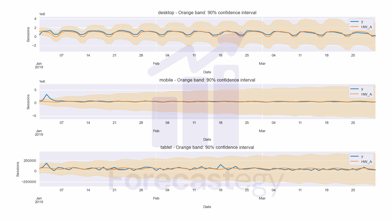
We can visually inspect the forecasts from the Holt-Winters model with additive errors:

And the forecasts from the Holt-Winters model with multiplicative errors:
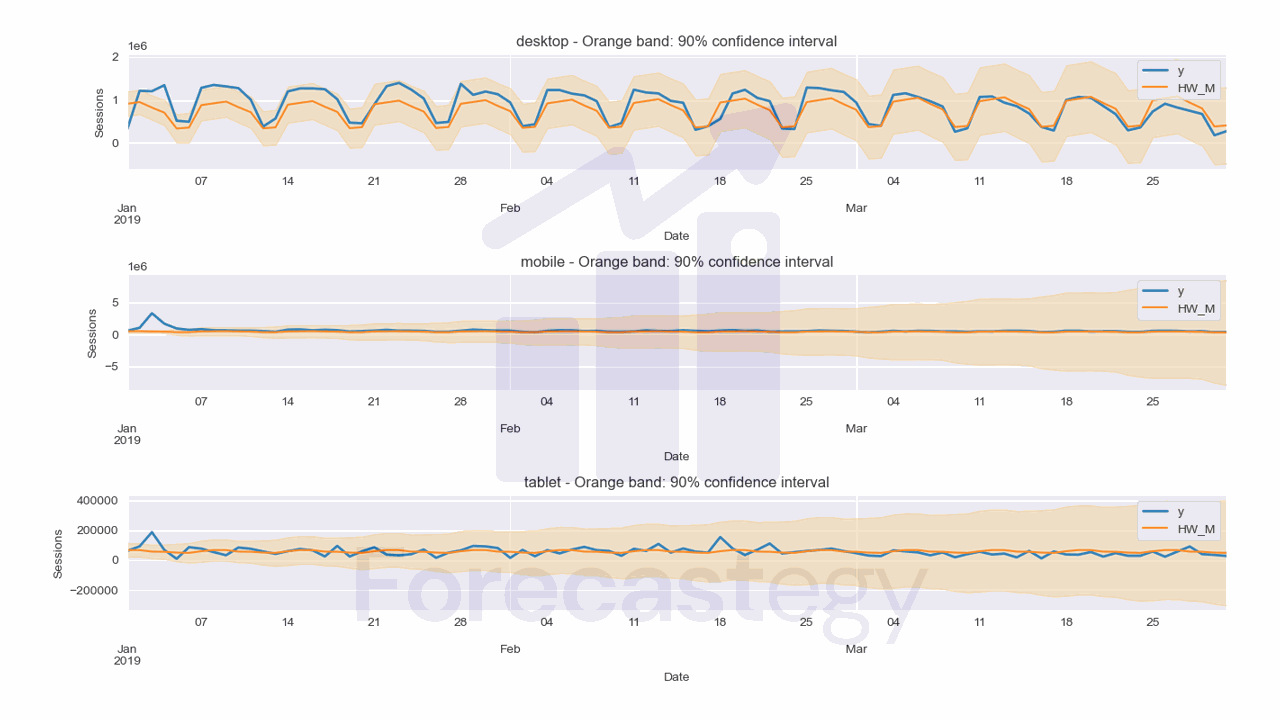
This is the code to plot the forecasts:
from sklearn.metrics import mean_absolute_percentage_error

for model_ in ['HW_A', 'HW_M']:
    mape_ = mean_absolute_percentage_error(p['y'].values, p[model_].values)
    print(f'{model_} MAPE: {mape_:.2%}')
    fig,ax = plt.subplots(3,1, figsize=(1280/96, 720/96))
    for ax_, device in enumerate(p['unique_id'].unique()):
        p.loc[p['unique_id'] == device].plot(x='ds', y='y', ax=ax[ax_], label='y', title=device, linewidth=2)
        p.loc[p['unique_id'] == device].plot(x='ds', y=model_, ax=ax[ax_], label=model_)
        ax[ax_].set_xlabel('Date')
        ax[ax_].set_ylabel('Sessions')
        ax[ax_].fill_between(p.loc[p['unique_id'] == device, 'ds'].values,
                            p.loc[p['unique_id'] == device, f'{model_}-lo-90'],
                            p.loc[p['unique_id'] == device, f'{model_}-hi-90'],
                            alpha=0.2,
                            color='orange')
        ax[ax_].set_title(f'{device} - Orange band: 90% prediction interval')
        ax[ax_].legend()
    fig.tight_layout()
    plt.show()
The mean_absolute_percentage_error function is from scikit-learn.
It’s a metric that measures the average percentage error between the actual and predicted values.
The Holt-Winters model with additive errors has a MAPE of 41.48%, while the Holt-Winters model with multiplicative errors has a MAPE of 33.38%.
I like the additive error model better when looking at the desktop plot, but the multiplicative error model is better in terms of MAPE.
So I would investigate the errors for each combination of model and device to see which models are better for each.
I would not be too concerned about overfitting here, but always use your domain knowledge to make the final decision.
StatsForecast contains many other traditional forecasting models, like ARIMA, that you can try next.
How To Use StatsModels To Train A Holt-Winters Models In Python
StatsForecast can be overkill if you just want to train a Holt-Winters model for a single time series.
In this case, you can use StatsModels, a popular Python library for statistical modeling.
We will try three different Exponential Smoothing models:
from statsmodels.tsa.holtwinters import SimpleExpSmoothing, Holt, ExponentialSmoothing

train_single_ts = train.loc[train['unique_id'] == 'desktop'].set_index('ds')['y']
valid_single_ts = valid.loc[valid['unique_id'] == 'desktop'].set_index('ds')['y']
To do this, I picked the desktop time series from the training and validation sets.
As we have only one series, we can easily convert it to a Pandas Series and set the date as the index.
This is very helpful to align the forecasts with the actual values for the validation set.
Simple Exponential Smoothing (SES)
This method is suitable for time series data without any trend or seasonality.
It uses a single smoothing factor to give more weight to recent observations.
The forecast formula for SES is given by:
$$F_{t+1} = \alpha Y_t + (1 - \alpha) F_t$$
Where $F_t$ is the forecast for period $t$, $Y_t$ is the actual observation for period $t$, and $\alpha$ is the smoothing factor ($0 \leq \alpha \leq 1$).
ses_model = SimpleExpSmoothing(train_single_ts).fit()

ses_forecast = ses_model.forecast(steps=h)

e = wmape(valid_single_ts, ses_forecast)
print(f"SES WMAPE: {e}")
The SimpleExpSmoothing class takes the time series as a parameter and returns a SimpleExpSmoothingResults object.
Different than the usual scikit-learn API, the fit method returns the fitted model.
With the fitted model, we can call the forecast method to get the forecasts.
The ses_forecast variable contains the forecasts for the validation set, preserving the index, starting from one period after the last date in the training set.
| y | |
|---|---|
| 2019-01-01 00:00:00 | 787777 |
| 2019-01-02 00:00:00 | 787777 |
| 2019-01-03 00:00:00 | 787777 |
| 2019-01-04 00:00:00 | 787777 |
| 2019-01-05 00:00:00 | 787777 |
Holt’s Linear Trend Method (HLT)
This method extends SES by adding another smoothing factor to capture the linear trend in the data.
The forecast and trend formulas for HLT are given by:
$$F_{t+1} = L_t + b_t$$
$$L_{t} = \alpha Y_t + (1 - \alpha)(L_{t-1} + b_{t-1})$$
$$b_t = \beta(L_{t} - L_{t-1}) + (1 - \beta)b_{t-1}$$
Where $F_t$ is the forecast for period $t$, $Y_t$ is the actual observation for period $t$, $L_t$ is the level at period $t$, $b_t$ is the trend at period $t$, $\alpha$ is the level smoothing factor ($0 \leq \alpha \leq 1$), and $\beta$ is the trend smoothing factor ($0 \leq \beta \leq 1$).
The code is very similar to the previous model:
hlt_model = Holt(train_single_ts).fit()

hlt_forecast = hlt_model.forecast(steps=h)

e = wmape(valid_single_ts, hlt_forecast)
print(f"HLT WMAPE: {e}")
Holt-Winters Exponential Smoothing (HWES)
This method further extends HLT by incorporating a third smoothing factor to handle seasonality in the data, similar to the Holt-Winters model we trained with StatsForecast.
The single step forecast formula for the additive HWES model is given by: $$F_{t+1} = L_t + b_t + S_{t - m + 1}$$
The level formula: $$L_t = \alpha (Y_t - S_{t-m}) + (1 - \alpha)(L_{t-1} + b_{t-1})$$
The trend formula: $$b_t = \beta (L_t - L_{t-1}) + (1 - \beta)b_{t-1}$$
The seasonal formula:: $$S_t = \gamma (Y_t - L_t) + (1 - \gamma)S_{t-m}$$
Where:
- $F_{t+1}$ is the forecast for period $t + 1$
- $Y_t$ is the actual observation for period $t$
- $L_t$ is the level at period $t$
- $b_t$ is the trend at period $t$
- $S_t$ is the seasonal component at period $t$
- $m$ is the number of periods in a seasonal cycle
- $\alpha$, $\beta$, and $\gamma$ are the level, trend, and seasonal smoothing factors with values between 0 and 1 ($0 \leq \alpha, \beta, \gamma \leq 1$)
hwes_model = ExponentialSmoothing(train_single_ts, seasonal='add', seasonal_periods=7).fit()

hwes_forecast = hwes_model.forecast(steps=h)

e = wmape(valid_single_ts, hwes_forecast)
print(f"HWES WMAPE: {e}")
Like in StatsForecast, we can set the seasonal parameter to add or mul to use additive or multiplicative seasonality, and the seasonal_periods parameter to the length of the season.
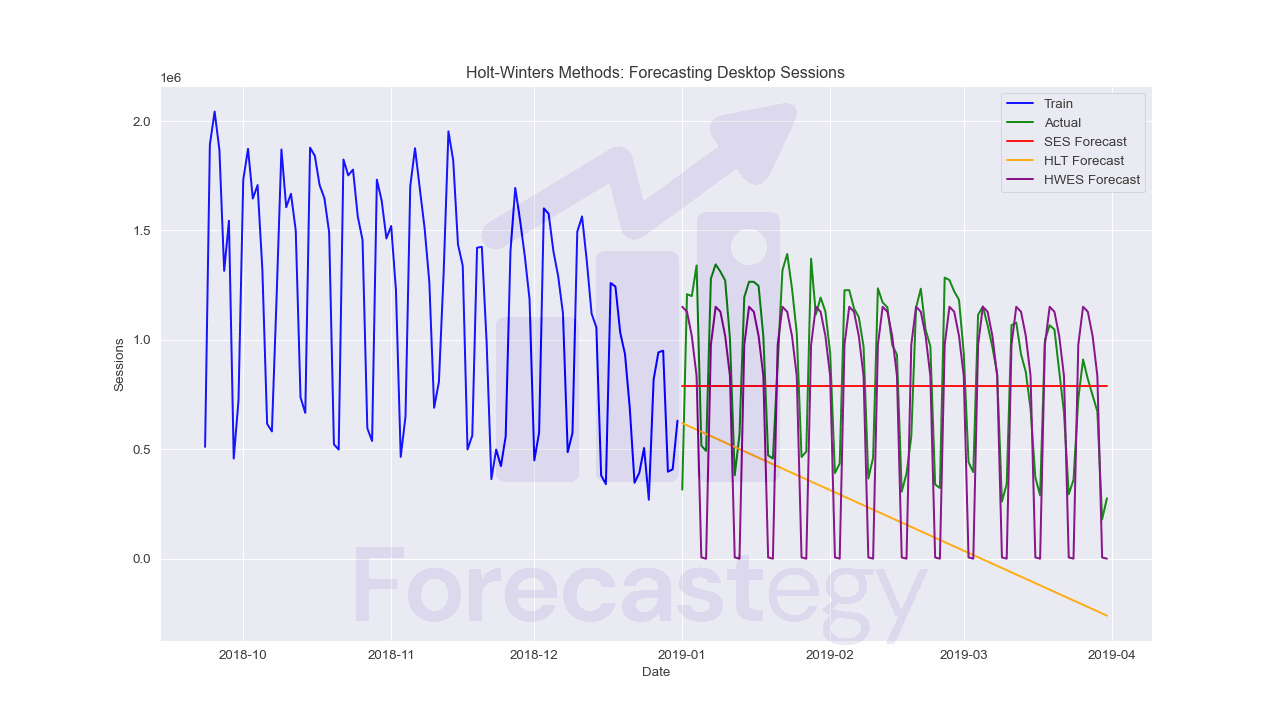
As you can see in the plot, seasonality is essential for this time series, so the last model is clearly the best.