Hierarchical forecasting is a method of forecasting time series data where the data is divided into multiple levels of aggregation.
The levels can be thought of as a tree-like structure, where each level represents a different aggregation of the data.
For example, the top level might represent total sales for a company, while the next level down might represent sales for each region, and the level below that might represent sales for each store within each region.
In some cases we want to create accurate forecasts for each level of the hierarchy, while ensuring that the forecasts at each level are consistent with the forecasts at the levels above and below.
This is where the concept of reconciling comes in.
Reconciliation is the process of combining forecasts from different levels of the hierarchy in a way that ensures consistency between the forecasts.
Reconciling forecasts is important for a number of reasons.
First, it can improve the accuracy of the forecasts by incorporating information from multiple levels of the hierarchy.
For example, if the forecasts for each store within a region are reconciled to the forecast for the region as a whole, the resulting forecast for the region is likely to be more accurate than if each store forecast was considered independently.
Second, reconciling forecasts can help to avoid inconsistencies and errors that can arise when forecasting each level independently.
For example, if the forecasts for each store within a region do not add up to the forecast for the region as a whole, this can lead to confusion and make it difficult to make decisions based on the forecasts.
In this tutorial, I will walk you through the steps of installing and using HierarchicalForecast, a fast and scalable Python library that will help you easily reconcile forecasts from multiple hierarchical levels.
Installing HierarchicalForecast
To install HierarchicalForecast, simply run the following command in your terminal:
pip install hierarchicalforecast
Or use conda:
conda install -c conda-forge hierarchicalforecast
HierarchicalForecast is responsible for the reconciliation part, after you have trained forecasting models for each level of the hierarchy and generated predictions.
To train models and generate predictions, you can use any method you like, such as scikit-learn, ARIMA, LSTM, or even naive methods.
I will use a simple Holt-Winters model.
Splitting Time Series Data Into Hierarchical Levels
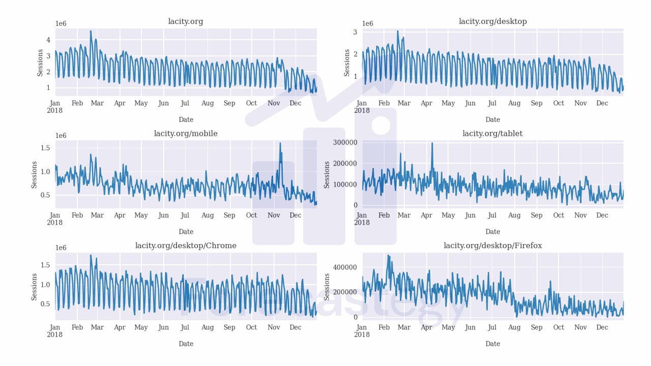
I will use data from the LACity.org website available on Kaggle.
This dataset contains the number of user sessions for the City of Los Angeles website for each day from 2014 to 2019.
Sessions are periods of time when a user is actively using the website.
Usually they are measured by looking at user activity and have a timeout after 30 minutes since the last user action.
For example, right now you are in a session on my website. If you leave the page and come back after 2 hours, you will be in a new session.
import pandas as pd
import numpy as np
from matplotlib import pyplot as plt
import os

data = pd.read_csv(os.path.join(path, 'lacity.org-website-traffic.csv'),
                   parse_dates=['Date']).loc[:, ['Date', 'Device Category', 'Browser', 'Sessions']]
data['Website'] = 'lacity.org'
selected = ['Chrome', 'Firefox', 'Internet Explorer', 'Opera', 'Safari',
       'Android Browser', 'Safari (in-app)']
data = data.loc[data['Browser'].isin(selected), :]
data = data.rename(columns={'Date': 'ds', 'Sessions': 'y'})
This is what the raw data looks like:
| Date | Device Category | Browser | Sessions | Website |
|---|---|---|---|---|
| 2014-01-01 00:00:00 | desktop | Chrome | 934 | lacity.org |
| 2014-01-01 00:00:00 | desktop | Firefox | 761 | lacity.org |
| 2014-01-01 00:00:00 | desktop | Internet Explorer | 1107 | lacity.org |
| 2014-01-01 00:00:00 | desktop | Opera | 35 | lacity.org |
| 2014-01-01 00:00:00 | desktop | Safari | 554 | lacity.org |
We have the following levels: Website, Device Category and Browser.
The Website level is the top level, then we have Device Category and Browser as the next levels.
For example, you are visiting this website from Desktop or Mobile, and you are likely using one of Chrome, Firefox, Edge, Opera or Safari.
HierarchicalForecast and it’s sister libraries expect the data to have 3 columns:
ds: the timestamp of the observationy: the value of the observationunique_id: a unique identifier for each time series
So I renamed the original Date column to ds and the Sessions column to y.
The original dataset didn’t have the Website column, so I added it manually. Although it’s the same for all rows, it’s still required so we can evaluate the aggregated forecasts later.
This is the data after the preprocessing:
| ds | Device Category | Browser | y | Website |
|---|---|---|---|---|
| 2014-01-01 00:00:00 | desktop | Chrome | 934 | lacity.org |
| 2014-01-01 00:00:00 | desktop | Firefox | 761 | lacity.org |
| 2014-01-01 00:00:00 | desktop | Internet Explorer | 1107 | lacity.org |
| 2014-01-01 00:00:00 | desktop | Opera | 35 | lacity.org |
| 2014-01-01 00:00:00 | desktop | Safari | 554 | lacity.org |
As always, I will split the data into train and validation sets in a simple time series validation scheme.
train = data.loc[data['ds'] < '2019-01-01']
valid = data.loc[(data['ds'] >= '2019-01-01') & (data['ds'] < '2019-02-01')]
h = valid['ds'].nunique()
Our validation data has 31 days, so our forecast horizon h is 31.
Now let’s make a list of the columns that represent the different levels of the hierarchy.
spec = [['Website'],
        ['Website', 'Device Category'],
        ['Website', 'Device Category', 'Browser']]
We will use this list to split the data into different levels with the aggregate function.
from hierarchicalforecast.utils import aggregate

train_agg, S_train, tags = aggregate(train, spec)
valid_agg, _, _ = aggregate(valid, spec)
We need to pass two arguments to it: the original dataframe and the list of lists of columns that represent the different levels of the hierarchy.
I like to do it separately for the train and validation sets to avoid data leakage.
The function returns 3 objects:
The first (train_agg or valid_agg) is a huge dataframe with the original data split into different levels and stacked on top of each other.
This is a random sample of rows from the train_agg dataframe:
| unique_id | ds | y |
|---|---|---|
| lacity.org/mobile/Opera | 2015-08-03 00:00:00 | 11546 |
| lacity.org/tablet/Android Browser | 2016-05-01 00:00:00 | 0 |
| lacity.org/mobile/Android Browser | 2018-06-11 00:00:00 | 0 |
| lacity.org/desktop/Safari | 2016-09-21 00:00:00 | 139579 |
| lacity.org/tablet/Opera | 2018-06-21 00:00:00 | 0 |
| lacity.org/mobile/Internet Explorer | 2014-05-28 00:00:00 | 0 |
| lacity.org/desktop/Opera | 2015-11-23 00:00:00 | 0 |
| lacity.org/desktop | 2015-01-17 00:00:00 | 833387 |
| lacity.org | 2018-06-04 00:00:00 | 2.84359e+06 |
| lacity.org/desktop/Opera | 2016-08-05 00:00:00 | 0 |
Notice that aggregate removed the Device Category and Browser columns, and replaced them with the unique_id column.
In Nixtla’s forecasting libraries (which HierarchicalForecast is part of), the unique_id column is used to identify each separate time series, as told above.
Some of the time series are very seasonal and kind of easy to forecast, but others are more challenging.
The second object (S_train) is a summing matrix that indicates which series are aggregated into which other series.
| lacity.org/desktop/Chrome | lacity.org/desktop/Firefox | lacity.org/desktop/Internet Explorer | lacity.org/desktop/Opera | lacity.org/desktop/Safari | |
|---|---|---|---|---|---|
| lacity.org | 1 | 1 | 1 | 1 | 1 |
| lacity.org/desktop | 1 | 1 | 1 | 1 | 1 |
| lacity.org/mobile | 0 | 0 | 0 | 0 | 0 |
| lacity.org/tablet | 0 | 0 | 0 | 0 | 0 |
| lacity.org/desktop/Chrome | 1 | 0 | 0 | 0 | 0 |
For example, the first row indicates that the lacity.org series is the sum of all the other series.
If we do the dot product of a row with the values of the original series indicated in the columns, we get the value of the aggregated series.
tags is a dictionary that maps the original categories to the unique_id values.
{...,
    'Website/Device Category': array(['lacity.org/desktop', 'lacity.org/mobile', 'lacity.org/tablet'],
       dtype=object), ...}
Now we are ready to train the models.
Training Forecasting Models For Each Hierarchical Level
I will use the StatsForecast library to train our Holt-Winters models.
from statsforecast import StatsForecast
from statsforecast.models import HoltWinters
model = StatsForecast(models=[HoltWinters(season_length=7, error_type='A')],
                              freq='D', n_jobs=-1)
model.fit(train_agg)
This code will train a separate Holt-Winters model for each level of the hierarchy (each unique_id we have in the train_agg dataframe).
For more details on StatsForecast and Holt-Winters, please refer to the links above.
Like I said, you can use any forecasting library you want, as long as you can generate forecasts for each level of the hierarchy.
We use the forecast method to generate the necessary data.
p = model.forecast(h=h, fitted=True)
p_fitted = model.forecast_fitted_values()
The argument h is the forecast horizon, and fitted=True indicates that we want to generate forecasts for both the training and validation periods.
Remember to do this if you are using a different forecasting library.
The forecast_fitted_values method returns the fitted values for the training period.
This is what p looks like:
| unique_id | ds | HoltWinters |
|---|---|---|
| lacity.org | 2019-01-01 00:00:00 | 1.67954e+06 |
| lacity.org | 2019-01-02 00:00:00 | 1.81115e+06 |
| lacity.org | 2019-01-03 00:00:00 | 1.52177e+06 |
| lacity.org | 2019-01-04 00:00:00 | 1.13103e+06 |
| lacity.org | 2019-01-05 00:00:00 | 943.062 |
And this is what p_fitted looks like:
| unique_id | ds | y | HoltWinters |
|---|---|---|---|
| lacity.org | 2014-01-01 00:00:00 | 1.66275e+06 | 2.28172e+06 |
| lacity.org | 2014-01-02 00:00:00 | 3.14611e+06 | 1.64666e+06 |
| lacity.org | 2014-01-03 00:00:00 | 2.85295e+06 | 2.20869e+06 |
| lacity.org | 2014-01-04 00:00:00 | 1.74434e+06 | 1.2439e+06 |
| lacity.org | 2014-01-05 00:00:00 | 1.93406e+06 | 1.61387e+06 |
It’s the format expected by HierarchicalForecast.
Reconciling Forecasts From Different Hierarchical Levels
Now that we have trained forecasting models for each level of the hierarchy, we need to reconcile the forecasts to ensure that they are consistent with each other.
From simple to complex, there are five different reconciliation methods that I will cover in this post and tell you how to select the best one for your problem.
Bottom-Up Reconciliation
The bottom-up method starts by forecasting the time series at the lowest level of the hierarchy (e.g., at the browser level), and then aggregates the forecasts up the hierarchy to higher levels (e.g., to the website level).
Top-Down Reconciliation
The top-down method starts by forecasting the time series at the highest level of the hierarchy (e.g., the website), and then disaggregates the forecasts down the hierarchy to lower levels (e.g., to the device and browser levels).
MinTrace, Optimal Combination and Empirical Risk Minimization
The MinTrace, Optimal Combination and Empirical Risk Minimization try to go further by explicitly minimizing the errors of the reconciled forecasting through optimization.
You can find more details and papers about them in the links above.
Selecting The Best Forecast Reconciliation Method
As we have a train and validation period, we can use the validation period to select the best reconciliation method just like any other hyperparameter.
from hierarchicalforecast.methods import BottomUp, TopDown, MinTrace, ERM, OptimalCombination
from hierarchicalforecast.core import HierarchicalReconciliation

reconcilers = [BottomUp(),
               TopDown(method='forecast_proportions'),
               TopDown(method='average_proportions'),
               TopDown(method='proportion_averages'),
               MinTrace(method='ols', nonnegative=True),
               MinTrace(method='wls_struct', nonnegative=True),
               MinTrace(method='wls_var', nonnegative=True),
               MinTrace(method='mint_shrink', nonnegative=True),
               MinTrace(method='mint_cov', nonnegative=True),
               OptimalCombination(method='ols', nonnegative=True),
               OptimalCombination(method='wls_struct', nonnegative=True),
               ERM(method='closed'),
               ERM(method='reg'),
               ERM(method='reg_bu'),
              ]

rec_model = HierarchicalReconciliation(reconcilers=reconcilers)

p_rec = rec_model.reconcile(Y_hat_df=p, Y_df=p_fitted, S=S_train, tags=tags)
HierarchicalForecast makes it very easy to train and compare different reconciliation methods.
We first need a list of the methods we want to try.
In this case I took the five we discussed above, with the allowed parameters plus an indicator that we want to use non-negative forecasts when possible.
Then we create a HierarchicalReconciliation object and pass the list of reconciliation methods to the reconcilers argument.
Finally, we use the reconcile method to reconcile the forecasts.
This method requires the following arguments:
Y_hat_df: the forecasts generated by the forecasting models for each level of the hierarchy in the validation period.Y_df: the predictions for the observations in the training period.S: the summing matrixtags: the mapping of each level of the hierarchy to the original categories.
This runs very fast, and it will return a dataframe with the forecasts for each reconciliation method.
| unique_id | ds | HoltWinters | HoltWinters/BottomUp | HoltWinters/TopDown_method-forecast_proportions | HoltWinters/TopDown_method-average_proportions |
|---|---|---|---|---|---|
| lacity.org | 2019-01-01 00:00:00 | 1.67954e+06 | 1.63374e+06 | 1.67954e+06 | 1.67954e+06 |
| lacity.org | 2019-01-02 00:00:00 | 1.81115e+06 | 1.63167e+06 | 1.81115e+06 | 1.81115e+06 |
| lacity.org | 2019-01-03 00:00:00 | 1.52177e+06 | 1.43171e+06 | 1.52177e+06 | 1.52177e+06 |
| lacity.org | 2019-01-04 00:00:00 | 1.13103e+06 | 1.13859e+06 | 1.13103e+06 | 1.13103e+06 |
| lacity.org | 2019-01-05 00:00:00 | 943.062 | 141860 | 943.062 | 943.062 |
I limited the columns here, but there is a column with the forecast of each reconciliation method.
I merged the forecasts with the actual values to compute the errors.
p_rec_ = p_rec.merge(valid_agg, on=['ds', 'unique_id'], how='left')
p_rec_['y'] = p_rec_['y'].fillna(0)
p_rec_ = p_rec_.reset_index(drop=False)

from sklearn.metrics import mean_squared_error

rmse = dict()
for model_ in p_rec.columns[1:]:
    rmse_ = mean_squared_error(p_rec_['y'].values, p_rec_[model_].values, squared=False)/1e3
    # get only the model name
    model__ = model_.split('/')[-1]
    rmse[model__] = rmse_
pd.DataFrame(rmse, index=['RMSE']).T.sort_values('RMSE')
You can use any metric you want, but I will use the RMSE as an example.
After computing the RMSE for each reconciliation method, I sorted it from the lowest to the highest.
(Values are divided by 1,000 to make it easier to read.)
| RMSE | |
|---|---|
| MinTrace_method-mint_shrink_nonnegative-True | 210.327 |
| MinTrace_method-wls_var_nonnegative-True | 211.071 |
| MinTrace_method-wls_struct_nonnegative-True | 211.715 |
| OptimalCombination_method-wls_struct_nonnegative-True | 211.715 |
| MinTrace_method-ols_nonnegative-True | 215.173 |
For this dataset, the MinTrace method with the mint_shrink parameter gave us the lowest error.
As always, evaluate more than one metric and use your domain knowledge as a prior to help you select the best reconciliation method.
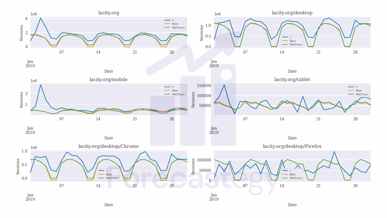
These are some of the forecasts for a few series:

In blue we have the actual values, in orange the forecasts from the Base model, which is the Holt-Winters over the raw series and in green the forecasts after reconciling with the selected MinTrace method.