ARIMA is one of the most popular univariate statistical models used for time series forecasting.
Here you will learn how to use the StatsForecast library, which provides a fast, scalable and easy-to-use interface for us to train ARIMA models in Python.
To understand ARIMA, let’s take an example of sales forecasting.
Suppose a retail store has historical sales data for the past 12 months.
To make a sales forecast for the next 3 months, we can fit an ARIMA model to this data.
The “autoregressive” (AR) component takes into account the autocorrelation structure of the data, which refers to the relation between the current value and the past values.
The “integrated” (I) component handles the non-stationarity in the data, that is, it applies differencing to make the mean and variance of the data constant across time.
The “moving average” (MA) component models the residuals or errors after removing the autocorrelation structure.
By default ARIMA doesn’t have a seasonal component, but we can add it by using SARIMA, which is one of the options provided by StatsForecast.
How To Install StatsForecast
StatsForecast is available on PyPI, so you can install it with pip:
pip install statsforecast
Or with conda:
conda install -c conda-forge statsforecast
How To Prepare The Data For StatsForecast ARIMA
We will use real sales data from the Favorita store chain, from Ecuador.
We have sales data from 2013 to 2017 for multiple stores and product categories.
To measure the model’s performance, we will use WMAPE (Weighted Mean Absolute Percentage Error) with the absolutes of the actual values as weights.
This is an adapted version of MAPE (Mean Absolute Percentage Error) that solves the problem of division by zero when there are no sales for a specific day.
import pandas as pd
import numpy as np
from matplotlib import pyplot as plt

def wmape(y_true, y_pred):
    return np.abs(y_true - y_pred).sum() / np.abs(y_true).sum()
For this tutorial I will use only the data from one store and two product categories.
You can use as many categories, SKUs, stores, etc as you want.
path = 'train.csv'
data = pd.read_csv(path, index_col='id', parse_dates=['date'])

data2 = data.loc[(data['store_nbr'] == 1) & (data['family'].isin(['MEATS', 'PERSONAL CARE'])), ['date', 'family', 'sales']]
The columns are:
date: date of the recordfamily: product categorysales: sales amount
StatsForecast expects the columns to be named in the following format:
ds: date of the recordy: target variable (sales amount)unique_id: unique identifier of the time series (product category)
So let’s rename them:
data2 = data2.rename(columns={'date': 'ds', 'sales': 'y', 'family': 'unique_id'})
unique_id should identify each time series you have.
If we had more than one store, we would have to add the store number along with the categories to unique_id.
An example would be unique_id = store_nbr + '_' + family.
This is the final version of our dataframe data2:
| ds | unique_id | y |
|---|---|---|
| 2013-01-01 00:00:00 | MEATS | 0 |
| 2013-01-01 00:00:00 | PERSONAL CARE | 0 |
| 2013-01-02 00:00:00 | MEATS | 369.101 |
| 2013-01-02 00:00:00 | PERSONAL CARE | 194 |
| 2013-01-03 00:00:00 | MEATS | 272.319 |
A row for each record containing the date, the time series ID (family in our example) and the target value.
Notice the time series records are stacked on top of each other.
Let’s split the data into train and validation sets.
How To Split Time Series Data For Validation
You should never use random or k-fold validation for time series.
That would cause data leakage, as you would be using future data to train your model.
In practice, you can’t take random samples from the future to train your model, so you can’t use them here.
To avoid this issue, we will use a simple time series split between past and future.
A career tip: knowing how to do time series validation correctly is a skill that will set you apart from many data scientists (even experienced ones!).
Our training set will be all the data between 2013 and 2016 and our validation set will be the first 3 months of 2017.
train = data2.loc[data2['ds'] < '2017-01-01']
valid = data2.loc[(data2['ds'] >= '2017-01-01') & (data2['ds'] < '2017-04-01')]
h = valid['ds'].nunique()
h is the horizon, the number of periods we want to forecast.
Note About This Data
This data doesn’t contain a record for December 25, so I just copied the sales from December 18 to December 25.
Without this step, the model would have a hard time capturing seasonality as it looks for a pattern that repeats every season_length records inside a series.
dec25 = list()
for year in range(2013,2017):
    dec25 += [{'ds': pd.Timestamp(f'{year}-12-25'), 'unique_id': 'MEATS', 'y': train.loc[(train['ds'] == f'{year}-12-18') & (train['unique_id'] == 'MEATS'), 'y'].values[0]},
            {'ds':  pd.Timestamp(f'{year}-12-25'), 'unique_id': 'PERSONAL CARE', 'y': train.loc[(train['ds'] == f'{year}-12-18') & (train['unique_id'] == 'PERSONAL CARE'), 'y'].values[0]}]
train = pd.concat([train, pd.DataFrame(dec25)], ignore_index=True).sort_values('ds')
How To Train ARIMA Models In Python With StatsForecast
Now we are ready to train our ARIMA models over all the time series in our training set.
from statsforecast import StatsForecast
from statsforecast.models import AutoARIMA

model = StatsForecast(models=[AutoARIMA(season_length=7)], freq='D', n_jobs=-1)
model.fit(train)
We are using the AutoARIMA object, which automatically selects the best ARIMA model for each time series.
Most time series data have a seasonal component, so we are using season_length=7 to indicate that the seasonality in this series is weekly.
We are also using n_jobs=-1 to use all the available cores in our machine.
We need to indicate the frequency of the data with freq='D' because we have daily data.
There are many other arguments we can use to customize the model, but leaving them as default is a good starting point.
p = model.predict(h=h, level=[90])
p = p.reset_index().merge(valid, on=['ds', 'unique_id'], how='left')

wmape_ = wmape(p['y'].values, p['AutoARIMA'].values)
print(f'WMAPE: {wmape_:.2%}')
To make predictions, we use the predict method with the horizon h and the confidence level level.
We can ask for multiple confidence levels at the same time by just adding their values to the list.
The horizon starts from the last date in the training set.
In our case, the last date in the training set is 2016-12-31, so the first prediction will be for 2017-01-01.
The predictions are stored in a dataframe with the following format:
| unique_id | ds | AutoARIMA | AutoARIMA-lo-90 | AutoARIMA-hi-90 | y |
|---|---|---|---|---|---|
| MEATS | 2017-01-01 00:00:00 | 139.747 | 9.81994 | 269.674 | 0 |
| PERSONAL CARE | 2017-01-01 00:00:00 | 114.05 | 56.252 | 171.847 | 0 |
| PERSONAL CARE | 2017-01-02 00:00:00 | 130.008 | 68.2149 | 191.801 | 81 |
| MEATS | 2017-01-02 00:00:00 | 252.643 | 121.801 | 383.486 | 116.724 |
| MEATS | 2017-01-03 00:00:00 | 277.937 | 146.709 | 409.164 | 344.583 |
It contains the stacked predictions for all the time series with columns for the point forecast, the lower and upper bounds of the confidence interval.
I merged the target values y with the predictions to make it easier to calculate the WMAPE and plot.
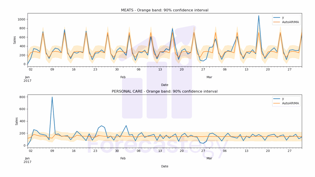
The WMAPE for this model is 21.19%
Let’s inspect the predictions visually to see if they make sense.
fig,ax = plt.subplots(2,1, figsize=(1280/96, 720/96))
for ax_, family in enumerate(['MEATS', 'PERSONAL CARE']):
    p.loc[p['unique_id'] == family].plot(x='ds', y='y', ax=ax[ax_], label='y', title=family, linewidth=2)
    p.loc[p['unique_id'] == family].plot(x='ds', y='AutoARIMA', ax=ax[ax_], label='AutoARIMA')
    ax[ax_].set_xlabel('Date')
    ax[ax_].set_ylabel('Sales')
    ax[ax_].fill_between(p.loc[p['unique_id'] == family, 'ds'].values,
                         p.loc[p['unique_id'] == family, 'AutoARIMA-lo-90'],
                         p.loc[p['unique_id'] == family, 'AutoARIMA-hi-90'],
                         alpha=0.2,
                         color='orange')
    ax[ax_].set_title(f'{family} - Orange band: 90% confidence interval')
    ax[ax_].legend()
fig.tight_layout()

By default the AutoARIMA object will use the best model it found according to the Akaike Information Criterion (AIC), just like other ARIMA packages across R and Python.
This is not necessarily the best model to minimize the metric you care about, but it’s a good model to have as a baseline.
The cool thing is that ARIMA models give us a confidence interval for the predictions, which is more useful than a simple point forecast in practice.
If more complex models (like LSTMs and scikit-learn models) can’t beat this simple model, you definitely should not deploy them.
Is ARIMA a Machine Learning Algorithm?
ARIMA can be considered a machine learning algorithm, albeit a very simple one.
Critics might argue that ARIMA, being a traditional statistical model, doesn’t fit into the machine learning category because it doesn’t involve more modern and complex techniques typically associated with machine learning.
Although it is a statistical method, it follows a similar process as other machine learning algorithms, which is to fit parameters and learn patterns from historical data to make predictions.
Another criticism might be that ARIMA’s focus on time series data makes it less versatile than other machine learning algorithms that can handle various types of data, such as images, text, or audio.
ARIMA’s specialization in time series analysis can be seen as a strength rather than a limitation because it serves a specific purpose and does it well.