In this blog post, I will walk you through a complete example of how to use Prophet for multiple time series forecasting.
Prophet, developed by Facebook (Meta) is an alternative to popular univariate time series models like ARIMA, that is claimed to be better for business use cases.
I will teach everything from installing Prophet to saving a trained model, and along the way, I will explain each step of the process in detail.
Let’s dive in!
Installing Prophet
Installing Prophet is very simple.
Do it via pip:
python -m pip install prophet
Or via conda:
conda install -c conda-forge prophet
Preparing the Data for Prophet
We will use real sales data from the Favorita store chain, from Ecuador.
We have sales data from 2013 to 2017 for multiple stores and product categories.
To measure the model’s performance, we will use WMAPE (Weighted Mean Absolute Percentage Error) with the absolutes of the actual values as weights.
import pandas as pd
import numpy as np

def wmape(y_true, y_pred):
    return np.abs(y_true - y_pred).sum() / np.abs(y_true).sum()
This is an adapted version of MAPE (Mean Absolute Percentage Error) that solves the problem of division by zero when there are no sales for a specific day.
For this tutorial I will use only the data from one store.
You can use as many stores, categories, SKUs, etc as you want.
data = pd.read_csv(os.path.join(path, 'train.csv'), index_col='id', parse_dates=['date'])
data2 = data.loc[data['store_nbr'] == 1, ['date', 'family', 'sales', 'onpromotion']]
The columns are:
date: date of the recordfamily: product categorysales: sales amountonpromotion: how many products of that category were on promotion on that day
This data doesn’t contain a record for December 25, so to test Prophet’s ability to handle missing values, I inserted a row with NaN values for that day.
dec25 = list()
for year in range(2013,2017):
    for family in data2['family'].unique():
        dec25 += [{'date': pd.Timestamp(f'{year}-12-25'), 'family': family, 'sales': np.nan, 'onpromotion': np.nan}]
data2 = pd.concat([data2, pd.DataFrame(dec25)], ignore_index=True).sort_values('date')
data2 = data2.rename(columns={'date': 'ds', 'sales': 'y'})
This is what the first 5 rows of data2 look like:
| ds | family | y | onpromotion |
|---|---|---|---|
| 2013-01-01 00:00:00 | AUTOMOTIVE | 0 | 0 |
| 2013-01-01 00:00:00 | SEAFOOD | 0 | 0 |
| 2013-01-01 00:00:00 | SCHOOL AND OFFICE SUPPLIES | 0 | 0 |
| 2013-01-01 00:00:00 | PRODUCE | 0 | 0 |
| 2013-01-01 00:00:00 | PREPARED FOODS | 0 | 0 |
One row per day per product category.
Prophet requires a minimum of two columns: the timestamp named ds and the value to forecast named y.
We have data from holidays in Ecuador and Prophet can use them to capture specific patterns around those days.
holidays_df = pd.read_csv(os.path.join(path, 'holidays_events.csv'))
holidays_df = holidays_df.loc[holidays_df['locale'] == 'National', ['date', 'description']]
holidays_df['lower_window'] = 0
holidays_df['upper_window'] = 0
holidays_df = holidays_df.rename(columns={'date': 'ds', 'description': 'holiday'})
This is what the first 5 rows of holidays_df look like:
| ds | holiday | lower_window | upper_window |
|---|---|---|---|
| 2012-08-10 | Primer Grito de Independencia | 0 | 0 |
| 2012-10-09 | Independencia de Guayaquil | 0 | 0 |
| 2012-10-12 | Traslado Independencia de Guayaquil | 0 | 0 |
| 2012-11-02 | Dia de Difuntos | 0 | 0 |
| 2012-11-03 | Independencia de Cuenca | 0 | 0 |
Prophet requires a column named ds with the date of the holiday and a column holiday with the name of the holiday.
The columns lower_window and upper_window specify how many days before and after the holiday to consider as influenced by the holiday in the model.
This is an useful feature to consider in any time series model.
Take, for example, the days before Christmas.
People tend to buy more gifts as the date approaches, so it’s important to capture that pattern in the model.
In Brazil, in the days before Carnival, people buy costumes and other items to celebrate the holiday. During it, people tend to buy more food and drinks.
As I don’t have the specific city of the stores, I will use only the national holidays.
Finally, we do a simple time series split into train and validation sets.
train = data2.loc[data2['ds'] < '2017-01-01']
valid = data2.loc[(data2['ds'] >= '2017-01-01') & (data2['ds'] < '2017-04-01')]
Training Prophet
We need to train a Prophet model for each time series we want to forecast.
Let’s learn to do it with a simple loop first and then we will parallelize it.
from prophet import Prophet

p = list()
for family in train['family'].unique():
    print('family:', family)
    train_ = train.loc[train['family'] == family]
    valid_ = valid.loc[valid['family'] == family]

    m = Prophet(seasonality_mode='additive', yearly_seasonality=True,
                weekly_seasonality=True, daily_seasonality=False,
                holidays=holidays_df)
    m.add_regressor('onpromotion')
    m.fit(train_)

    future = m.make_future_dataframe(periods=90, include_history=False)
    future = future.merge(valid_[['ds', 'onpromotion']], on='ds', how='left')
    forecast = m.predict(future)
    forecast['family'] = family
    p.append(forecast[['ds', 'yhat', 'family']])

p = pd.concat(p, ignore_index=True)
p['yhat'] = p['yhat'].clip(lower=0)
p = p.merge(valid, on=['ds', 'family'], how='left')
wmape(p['y'], p['yhat'])
We start by importing Prophet and creating a list p to store the predictions.
Then we have a loop that iterates over the unique values of the family column in the train dataset to create a separate forecast for each series.
Next, the code creates two new datasets, train_ and valid_, that contain only the rows of the original training and validation datasets that correspond to the current family being forecasted.
The next few lines create a new Prophet object called m and set a few parameters.
seasonality_mode is set to additive by default, but it could be set to multiplicative. This parameter controls how the seasonal components are modeled.
yearly_seasonality corresponds to seasonality across the entire year. It can be used to capture back-to-school seasonality, summer vacation seasonality, and so on.
weekly_seasonality models patterns that repeat across the week. It can be used to capture patterns like weekends being busier than weekdays.
daily_seasonality models patterns that repeat across the day. It can be used to capture patterns like lunchtime being busier than dinnertime.
The holidays parameter is set to holidays_df, which is our dataframe with information about the holidays in Ecuador.
Next, we use the function add_regressor to add the column onpromotion to the model. You can use this function to add as many external variables as you want to the model.
The function fit trains the model using the training data.
Next, the code creates a new dataframe called future that contains the dates for the next 90 days after the end of the train_ dataset.
I set the include_history parameter to False because I don’t want to include the dates from the training data in the future dataset.
This is what the first 5 rows of future look like at this point:
| ds |
|---|
| 2017-01-01 |
| 2017-01-02 |
| 2017-01-03 |
| 2017-01-04 |
| 2017-01-05 |
The next line adds the column onpromotion to the future dataset. This is necessary for the model to use the information about the promotions in the forecast.
If we had external variables that we could not plan in advance (like temperature or commodity prices), we would need to use estimates.
This is what the first 5 rows of future look like now:
| ds | onpromotion |
|---|---|
| 2017-01-01 00:00:00 | 0 |
| 2017-01-02 00:00:00 | 0 |
| 2017-01-03 00:00:00 | 0 |
| 2017-01-04 00:00:00 | 0 |
| 2017-01-05 00:00:00 | 0 |
Hours in the timestamp are not important for this model, but Pandas added it automatically.
Forecasting With Prophet
We use the function predict to make predictions for the dates in future.
The forecast variable is the dataframe with the predicted values for each date in the future dataframe.
This is the input dataframe for the predict function:
| ds | onpromotion |
|---|---|
| 2017-01-01 00:00:00 | 0 |
| 2017-01-02 00:00:00 | 0 |
| 2017-01-03 00:00:00 | 0 |
| 2017-01-04 00:00:00 | 0 |
| 2017-01-05 00:00:00 | 0 |
The prediction dataframe returned by the function contains many columns, but we will focus on the following:
| ds | yhat | yhat_lower | yhat_upper |
|---|---|---|---|
| 2017-01-01 00:00:00 | -0.398921 | -3.12561 | 2.52133 |
| 2017-01-02 00:00:00 | 4.8447 | 1.82306 | 7.55953 |
| 2017-01-03 00:00:00 | 5.70195 | 2.66954 | 8.71459 |
| 2017-01-04 00:00:00 | 5.14328 | 2.05284 | 8.22002 |
| 2017-01-05 00:00:00 | 4.60457 | 1.48575 | 7.53965 |
yhatis the midpoint of the prediction interval. It is the most likely value for the forecast.yhat_loweris the lower bound of the prediction interval.yhat_upperis the upper bound of the prediction interval.
Next, the code adds a new column to the forecast dataframe called family and sets its value to the name of the family that was just forecasted.
This step is important because the final p dataframe will contain predictions for multiple families, and we need to be able to distinguish between them.
The forecast dataframe is then appended to the p list.
This process is repeated for each family (series) in the dataset.
After all of the series have been forecasted, we use the pd.concat function to concatenate all of the dataframes in the p list into a single dataframe.
I clipped the values in the yhat column to be greater than or equal to 0 because the yhat column contains negative values, which don’t make sense for this dataset.
Sometimes you see negative values in the target variable for demand forecasting problems because it considers more items were returned than were sold.
If negative values make sense for your problem, you can skip this step.
Finally, we merge the p dataframe with the valid dataframe to calculate the WMAPE metric.
WMAPE was 17.19% for the validation set.
In practice, we compare this value with the WMAPE of a baseline model to see if the model is worth using.
These are the first 5 rows of the p dataframe:
| ds | yhat | family | y | onpromotion |
|---|---|---|---|---|
| 2017-01-01 00:00:00 | 0 | AUTOMOTIVE | 0 | 0 |
| 2017-01-01 00:00:00 | 0 | DAIRY | 0 | 0 |
| 2017-01-01 00:00:00 | 0 | SEAFOOD | 0 | 0 |
| 2017-01-01 00:00:00 | 28.1703 | HOME CARE | 0 | 0 |
| 2017-01-01 00:00:00 | 0 | BEAUTY | 0 | 0 |

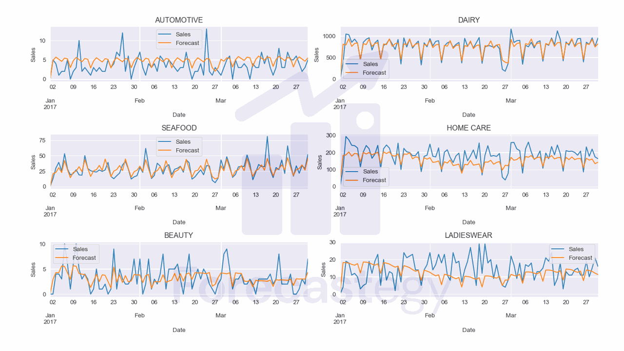
I used the following code to plot the forecast for a few families:
fig, ax = plt.subplots(3,2, figsize=(1280/96, 720/96), dpi=96)
ax = ax.flatten()
for ax_ ,family in enumerate(p['family'].unique()[:6]):
    p_ = p.loc[p['family'] == family]
    p_.plot(x='ds', y='y', ax=ax[ax_], label='Sales')
    p_.plot(x='ds', y='yhat', ax=ax[ax_], label='Forecast')
    ax[ax_].set_title(family)
    ax[ax_].legend()
    ax[ax_].set_xlabel('Date')
    ax[ax_].set_ylabel('Sales')
fig.tight_layout()
plt.show()
Parallelizing the Training And Prediction
We can make the training and prediction process MUCH faster by parallelizing it.
My favorite ways of doing it are using the joblib or dask libraries.
Here I will show you how to do it with joblib.
First we need to take the code from the loop and put it in a function.
from prophet import Prophet
from joblib import Parallel, delayed

def run_one(train_, valid_, family):
    print('family:', family)
    m = Prophet(seasonality_mode='additive', yearly_seasonality=True,
                weekly_seasonality=True, daily_seasonality=False,
                holidays=holidays_df)
    m.add_regressor('onpromotion')
    m.fit(train_)

    future = m.make_future_dataframe(periods=90, include_history=False)
    future = future.merge(valid_[['ds', 'onpromotion']], on='ds', how='left')
    forecast = m.predict(future)
    forecast['family'] = family
    return forecast[['ds', 'yhat', 'family']]
This function takes a training and validation set for a single family and returns a dataframe with the forecast. The third argument is the name of the family.
We could subset the train and valid dataframes inside the function, but sometimes doing it before helps us make less copies of the data in memory.
Next, we need to create a list of jobs to run in parallel.
jobs = list()
for family in train['family'].unique():
    train_ = train.loc[train['family'] == family]
    valid_ = valid.loc[valid['family'] == family]
    jobs.append(delayed(run_one)(train_, valid_, family))
First, we prepare the training and validation sets for each family.
Then we use the delayed function from the joblib library to create a job for each family.
We pass the run_one function as the argument and then pass the function arguments to a second set of parentheses.
This will not run the function, it will just create the jobs that we will run in parallel.
p = Parallel(n_jobs=4)(jobs)
p = pd.concat(p, ignore_index=True)
p['yhat'] = p['yhat'].clip(lower=0)
p = p.merge(valid, on=['ds', 'family'], how='left').sort_values('ds')
wmape(p['y'], p['yhat'])
We then call the Parallel object from the joblib library passing how many jobs we want to run in parallel as the n_jobs argument. Usually the number of jobs should be equal to the number of cores on your machine.
In the second set of parentheses, we pass the list of jobs that we created earlier.
Finally, with the p list of dataframes, we proceed with the same steps as before.
Saving a Prophet Model
If you want to save a Prophet model for later use, you can use tools from the serialize module inside the function we created.
The models are saved as JSON files.
from prophet.serialize import model_to_json, model_from_json

...
m.fit(train_)

with open(f'prophet_{family}.json', 'w') as f:
    f.write(model_to_json(m))

future = m.make_future_dataframe(periods=90, include_history=False)
...
Then, to load the model, you can use the following code:
with open(f'prophet_{family}.json', 'r') as f:
    m = model_from_json(f.read())
After loading you can use it as if you had just trained it.