What Is Naive Forecasting?
Whenever you start a time series forecasting project, you should start with a naive model.
A naive model is a very simple rule that you use to generate predictions for the future.
It’s easy to implement and it gives you a baseline to compare your more complex models against.
Here you will learn how to use the StatsForecast library, which provides the most popular naive models for time series forecasting in Python.
How To Install StatsForecast
StatsForecast is available on PyPI, so you can install it with pip:
pip install statsforecast
Or with conda:
conda install -c conda-forge statsforecast
What Are The Types Of Naive Forecasting Models
We will try the following naive models:
Simple Naive Forecast
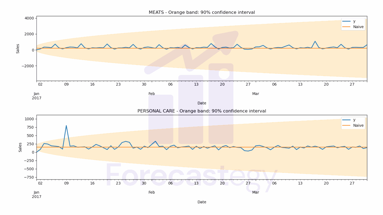
The simple naive model predicts the next values as the last observed value.
It’s that simple, just take the last value you have in your data and use it as the prediction for any future time steps.
This works because many time series have a recency bias, which means that the most recent values are more predictive than the older ones.
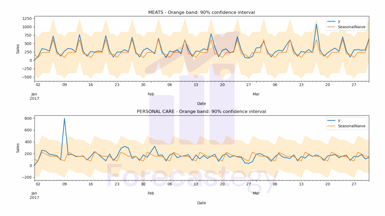
Seasonal Naive Forecast
The seasonal naive model takes the last observed value from a similar period in the past.
For example, if we want to know the sales for next Friday, we can use the sales from the previous week Friday.
This way we have a recent value, but slightly more sophisticated than the simple naive model.
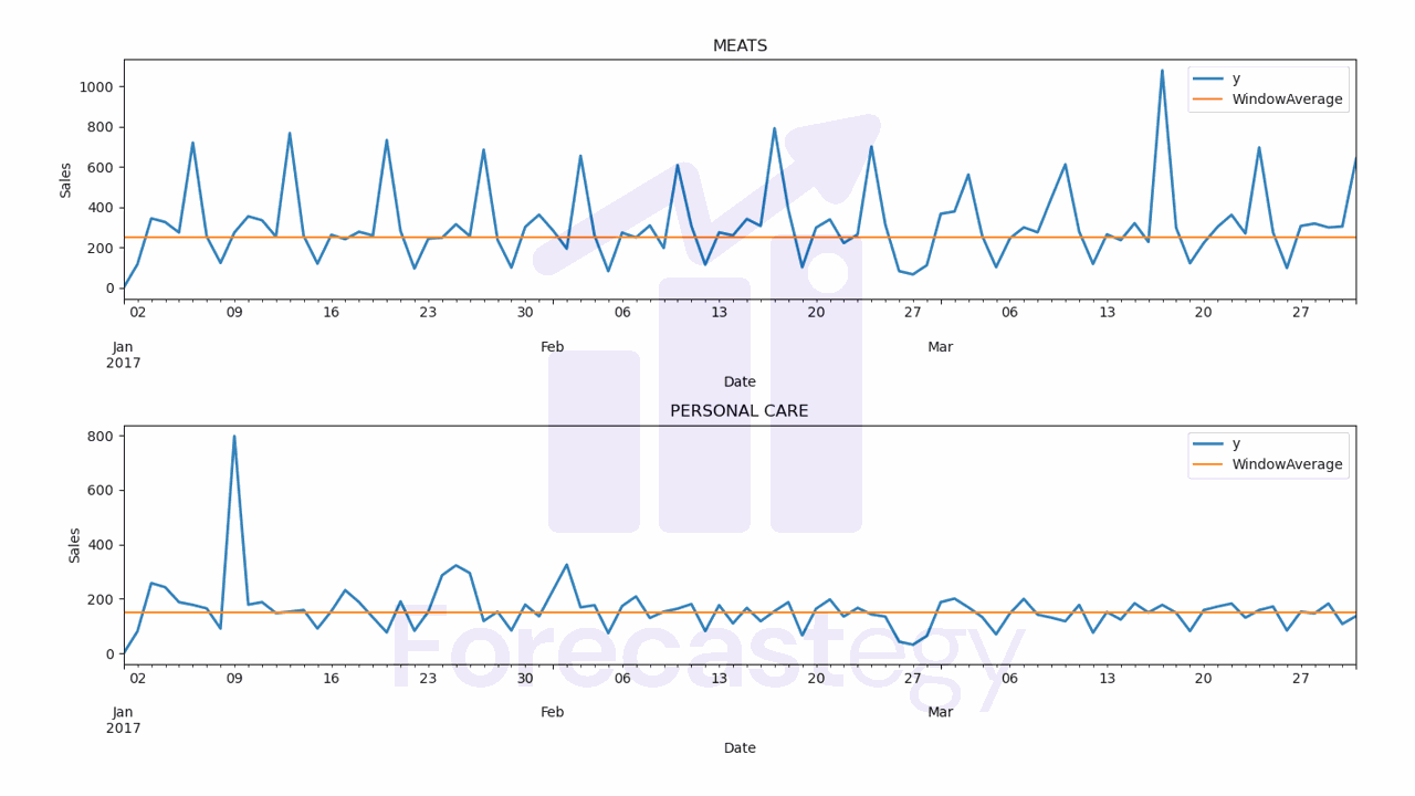
Window Average Forecast
The window average model takes the average of the last window_size values of the series.
Then it uses this average as the prediction for any future time steps.
It works by smoothing out the noise in the series.
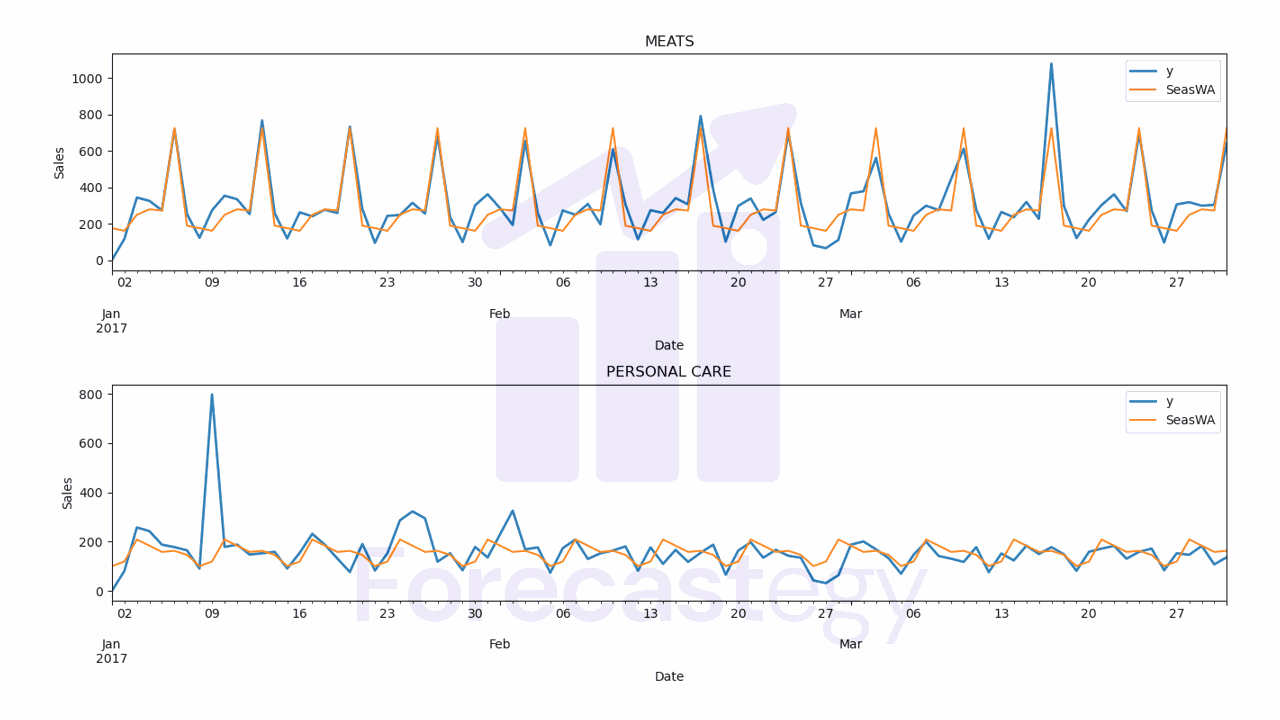
Seasonal Window Average Forecast
The seasonal window average model takes the average of the last window_size values from a similar period in the past.
In our Friday example, we would take the average of the sales from the previous window_size Fridays.
If we have a noisy but seasonal series, this model will be able to smooth out the noise and still capture the seasonality.
How To Prepare The Data For StatsForecast
We will use real sales data from the Favorita store chain, from Ecuador.
We have sales data from 2013 to 2017 for multiple stores and product categories.
To measure the model’s performance, we will use WMAPE (Weighted Mean Absolute Percentage Error) with the absolutes of the actual values as weights.
This is an adapted version of MAPE (Mean Absolute Percentage Error) that solves the problem of division by zero when there are no sales for a specific day.
import pandas as pd
import numpy as np
from matplotlib import pyplot as plt

def wmape(y_true, y_pred):
    return np.abs(y_true - y_pred).sum() / np.abs(y_true).sum()
For this tutorial I will use only the data from one store and two product categories.
You can use as many categories, SKUs, stores, etc as you want.
path = 'train.csv'
data = pd.read_csv(path, index_col='id', parse_dates=['date'])

data2 = data.loc[(data['store_nbr'] == 1) & (data['family'].isin(['MEATS', 'PERSONAL CARE'])), ['date', 'family', 'sales']]
The columns are:
date: date of the recordfamily: product categorysales: sales amount
StatsForecast expects the columns to be named in the following format:
ds: date of the recordy: target variable (sales amount)unique_id: unique identifier of the time series (product category)
So let’s rename them:
data2 = data2.rename(columns={'date': 'ds', 'sales': 'y', 'family': 'unique_id'})
unique_id should identify each time series you have.
If we had more than one store, we would have to add the store number along with the categories to unique_id.
An example would be unique_id = store_nbr + '_' + family.
This is the final version of our dataframe data2:
| ds | unique_id | y |
|---|---|---|
| 2013-01-01 00:00:00 | MEATS | 0 |
| 2013-01-01 00:00:00 | PERSONAL CARE | 0 |
| 2013-01-02 00:00:00 | MEATS | 369.101 |
| 2013-01-02 00:00:00 | PERSONAL CARE | 194 |
| 2013-01-03 00:00:00 | MEATS | 272.319 |
A row for each record containing the date, the time series ID (family in our example) and the target value.
Notice the time series records are stacked on top of each other.
Let’s split the data into train and validation sets.
How To Split Time Series Data For Validation
You should never use random or k-fold validation for time series.
That would cause data leakage, as you would be using future data to train your model.
In practice, you can’t take random samples from the future to train your model, so you can’t use them here.
To avoid this issue, we will use a simple time series split between past and future.
A career tip: knowing how to do time series validation correctly is a skill that will set you apart from many data scientists (even experienced ones!).
Our training set will be all the data between 2013 and 2016 and our validation set will be the first 3 months of 2017.
train = data2.loc[data2['ds'] < '2017-01-01']
valid = data2.loc[(data2['ds'] >= '2017-01-01') & (data2['ds'] < '2017-04-01')]
h = valid['ds'].nunique()
h is the horizon, the number of periods we want to forecast.
Note About This Data
This data doesn’t contain a record for December 25, so I just copied the sales from December 18 to December 25.
Without this step, the model would have a hard time capturing seasonality as it looks for a pattern that repeats every season_length records in the series.
dec25 = list()
for year in range(2013,2017):
    dec25 += [{'ds': pd.Timestamp(f'{year}-12-25'), 'unique_id': 'MEATS', 'y': train.loc[(train['ds'] == f'{year}-12-18') & (train['unique_id'] == 'MEATS'), 'y'].values[0]},
            {'ds':  pd.Timestamp(f'{year}-12-25'), 'unique_id': 'PERSONAL CARE', 'y': train.loc[(train['ds'] == f'{year}-12-18') & (train['unique_id'] == 'PERSONAL CARE'), 'y'].values[0]}]
train = pd.concat([train, pd.DataFrame(dec25)], ignore_index=True).sort_values('ds')
How To Build Naive Forecasting Models In Python
It’s very easy to build naive forecasting models using StatsForecast.
from statsforecast import StatsForecast
from statsforecast.models import Naive, SeasonalNaive, WindowAverage, SeasonalWindowAverage

model = StatsForecast(models=[Naive(),
                              SeasonalNaive(season_length=7),
                              WindowAverage(window_size=7),
                              SeasonalWindowAverage(window_size=2, season_length=7)],
                      freq='D', n_jobs=-1)
model.fit(train)
We pass a list of models to the models argument of the StatsForecast class.
Here we are using the models described above: Naive, SeasonalNaive, WindowAverage and SeasonalWindowAverage.
For the SeasonalNaive and SeasonalWindowAverage models, we need to specify the season length, which in our case is weekly, so 7 periods.
For the WindowAverage and SeasonalWindowAverage models, we need to specify the window size, which I arbitrarily chose to be 7 and 2 periods.
This means that the WindowAverage model will use the average of the last 7 days of the training data to make the prediction and the SeasonalWindowAverage model will use the average of specific days in the last 2 weeks.
In practice you must try different window sizes and season lengths to find the ones that minimize the evaluation metric in your validation set.
The freq argument is the frequency of the data, in our case daily
The n_jobs argument is the number of cores to use for parallelization.
Now we can make predictions for the steps after the last date in the training set.
p = model.predict(h=h, level=[90])
p = p.reset_index().merge(valid, on=['ds', 'unique_id'], how='left')
In our case, the last date in the training set is 2016-12-31, so the first prediction will be for 2017-01-01.
I merged the target values y with the predictions to make it easier to calculate the WMAPE and plot.
The predictions are stored in a dataframe with the following format:
| unique_id | ds | Naive | Naive-lo-90 | Naive-hi-90 | SeasonalNaive | SeasonalNaive-lo-90 | SeasonalNaive-hi-90 | WindowAverage | SeasWA | y |
|---|---|---|---|---|---|---|---|---|---|---|
| MEATS | 2017-01-01 00:00:00 | 187.434 | -201.434 | 576.302 | 176.26 | -435.263 | 787.783 | 251.709 | 176.26 | 0 |
| PERSONAL CARE | 2017-01-01 00:00:00 | 150 | 57.1832 | 242.817 | 101 | -175.316 | 377.316 | 150.143 | 101 | 0 |
| PERSONAL CARE | 2017-01-02 00:00:00 | 150 | 18.7373 | 281.263 | 74 | -202.316 | 350.316 | 150.143 | 119.5 | 81 |
| MEATS | 2017-01-02 00:00:00 | 187.434 | -362.508 | 737.376 | 80.884 | -530.639 | 692.407 | 251.709 | 161.769 | 116.724 |
| MEATS | 2017-01-03 00:00:00 | 187.434 | -486.104 | 860.972 | 229.281 | -382.242 | 840.804 | 251.709 | 249.757 | 344.583 |
It contains the stacked predictions for all the time series with columns for all the models.
Naive and SeasonalNaive have confidence intervals, the other models don’t.
The WMAPE for each model is:
- Naive WMAPE: 44.00%
- SeasonalNaive WMAPE: 29.78%
- WindowAverage WMAPE: 36.48%
- SeasWA WMAPE: 24.22%
Let’s inspect the predictions visually to see if they make sense.
for model_ in ['Naive', 'SeasonalNaive', 'WindowAverage', 'SeasWA']:
    fig,ax = plt.subplots(2,1, figsize=(1280/96, 720/96))
    for ax_, family in enumerate(['MEATS', 'PERSONAL CARE']):
        p.loc[p['unique_id'] == family].plot(x='ds', y='y', ax=ax[ax_], label='y', title=family, linewidth=2)
        p.loc[p['unique_id'] == family].plot(x='ds', y=model_, ax=ax[ax_], label=model_)
        ax[ax_].set_xlabel('Date')
        ax[ax_].set_ylabel('Sales')
        if model_ in ['Naive', 'SeasonalNaive']:
            ax[ax_].fill_between(p.loc[p['unique_id'] == family, 'ds'].values,
                                p.loc[p['unique_id'] == family, f'{model_}-lo-90'],
                                p.loc[p['unique_id'] == family, f'{model_}-hi-90'],
                                alpha=0.2,
                                color='orange')
            ax[ax_].set_title(f'{family} - Orange band: 90% confidence interval')
        ax[ax_].legend()
    fig.tight_layout()
    wmape_ = wmape(p['y'].values, p[model_].values)
    print(f'{model_} WMAPE: {wmape_:.2%}')

Now you can try increasingly complex models like ARIMA, Kalman Filters, neural networks and even ensemble models and see if they can beat the WMAPE.