
A fast, easy, and hands-off approach to creating ensemble models for time series forecasting is using AutoGluon.
AutoGluon is an open-source AutoML library for deep learning.
It’s a great tool for time series forecasting because it can automatically select the best models for your data and ensemble them together to create a more accurate model.
It also has a built-in feature to handle missing values and can handle large datasets.
We’ll start by installing AutoGluon and setting it up, before delving into a hands-on example using real-world data from the Los Angeles City website.
To get the most out of this tutorial, you should have a basic understanding of Python and machine learning concepts.
But don’t worry if you’re not an expert – I’ll walk you through each step with clear explanations and practical applications.
By the end of this tutorial, you’ll have a solid grasp on how to leverage AutoGluon for time series forecasting in Python and create powerful ensemble models.
What Is An Ensemble Model In Time Series Forecasting?
Let’s imagine you’re in charge of predicting the sales of a certain product for the next year.
Making these predictions accurately is super important to ensure there’s enough stock to meet customer demand, but not so much that it sits around gathering dust.
One way to make these predictions is by using time series forecasting models.
An ensemble is basically a group of these forecasting models working together, like a team, to make even better predictions.
By combining the strengths and insights of different models, an ensemble is usually able to provide forecasts that are more accurate than any single model working alone.
It’s a bit like asking several friends for their opinions on something – by listening to all of their perspectives, you’ll likely make a more informed decision.
Why Use An Ensemble In Time Series Forecasting?
Ensembles of time series forecasting models are useful because they allow us to extract more information from our data and to capture different trends and patterns that might have been missed by a single model.
For example, one model might be really good at identifying overall trends, while another might excel at picking up on seasonal changes.
By combining these models in an ensemble, we can leverage their unique strengths and create a more accurate forecast.
When To Use Or Not Use An Ensemble?
These ensembles are best used when the data you’re working with is complex and you need to extract as much information as possible from it.
If having a half-percentage point improvement in accuracy is worth the extra effort, then an ensemble is a great choice.
However, it’s important to recognize when an ensemble might not be the best choice.
If your data is quite simple, and a single model can do a good job of capturing the patterns in it, then an ensemble might just be overkill.
Install AutoGluon For Time Series Forecasting
First, you should install AutoGluon according to your operating system (OS) and decide if you want to use a GPU or not.
Follow the instructions on the AutoGluon website.
For Windows users, you may need to install PyTorch and CUDA first and then install AutoGluon.
To check if your installation with CUDA is successful, run the following code:
import torch
print(torch.cuda.is_available())
It must return True.
Loading Time Series Data
I will use data from the Los Angeles City website to demonstrate how to use AutoGluon for time series forecasting.
This dataset contains the number of visits per day for different devices (desktop, mobile, tablet) from 2016 to 2019.
We are going to use sessions as our target variable. A session is a group of interactions that take place on a website within a given time frame.
For example, right now you are reading this article, and this is one session. Everything you do on the next minutes will be part of this session.
If you come back to this article later, it will be a new session.
import pandas as pd
import numpy as np
from matplotlib import pyplot as plt
import os

data = pd.read_csv(os.path.join(path, 'lacity.org-website-traffic.csv'),
                   parse_dates=['Date']).loc[:, ['Date', 'Device Category', 'Sessions']]
data = data.groupby(['Date', 'Device Category'], as_index=False)['Sessions'].sum()

# missing dates
fixes = pd.DataFrame({'Date': pd.to_datetime(['2016-12-01', '2018-10-13']),
                      'Device Category': ['tablet', 'tablet'] ,
                      'Sessions': [np.nan, np.nan]})

data = pd.concat([data, fixes], axis=0, ignore_index=True)
data = data.rename(columns={'Device Category': 'item_id', 'Sessions': 'target', 'Date': 'timestamp'})
# backfill
data = data.sort_values(['item_id', 'timestamp']).groupby('item_id').apply(lambda x: x.fillna(method='ffill'))

train = data[data.timestamp < '2019-01-01']
valid = data[(data.timestamp >= '2019-01-01') & (data.timestamp < '2019-02-01')]
Your data must be in the “long” format, where each row represents a single observation.
It’s good practice to rename the columns to timestamp and target to make it easier to work with the library.
By renaming the 'Device Category' column to 'item_id', it indicates that this is the column which maps each row to a unique time series.
Similarly, renaming the 'Sessions' column to 'target' emphasizes that this column contains the values we aim to predict in our time series forecasting.
Additionally, renaming the 'Date' column to 'timestamp' makes it clear that this column contains the timestamp information for each data point in the time series.
These standardized names help in maintaining consistency and improve code readability throughout the analysis.
Although AutoGluon splits the data into train and validation sets internally, I like to have an external validation set to make sure we are not overfitting after training the model and ensemble.
The library requires the data to be in a specific format:
from autogluon.timeseries import TimeSeriesDataFrame, TimeSeriesPredictor

train_ag = TimeSeriesDataFrame.from_data_frame(train, timestamp_column='timestamp', id_column='item_id')
valid_ag = TimeSeriesDataFrame.from_data_frame(valid, timestamp_column='timestamp', id_column='item_id')
This code is responsible for importing the necessary classes and converting the training and validation Pandas DataFrames into TimeSeriesDataFrame objects, which are specifically designed for time series analysis in AutoGluon.
Here’s a breakdown of the important lines in the code:
train_ag = TimeSeriesDataFrame.from_data_frame(train, timestamp_column='timestamp', id_column='item_id')
In this line, we’re converting the train DataFrame into a TimeSeriesDataFrame object called train_ag.
We pass the train DataFrame to the from_data_frame() method and specify the 'timestamp_column' and 'id_column' parameters.
The timestamp_column parameter tells the method which column in the DataFrame contains the timestamps.
The id_column parameter is used to specify the column that contains the mapping of rows to time series in the dataset.
AutoGluon can handle multiple time series in the same dataset, so we need to specify the column that contains the unique identifiers for each.
In our case, we want to treat each device as an “independent” time series, so we renamed the 'Device Category' column to 'item_id'.
valid_ag = TimeSeriesDataFrame.from_data_frame(valid, timestamp_column='timestamp', id_column='item_id')
Similarly, this line converts the valid DataFrame into a TimeSeriesDataFrame object named valid_ag.
Just like with the train DataFrame, we pass the valid DataFrame to the from_data_frame() method and specify the 'timestamp_column' and 'id_column' parameters.
Training The Forecasting Models And Ensemble
predictor = TimeSeriesPredictor(prediction_length=30, target='target', eval_metric='MAPE')

predictor.fit(
    train_ag,
    presets="medium_quality",
    time_limit=600,
)
In this step, we create and train a time series forecasting model using AutoGluon’s TimeSeriesPredictor class.
The TimeSeriesPredictor is designed for handling the training and prediction processes of time series models with various configurations.
First, we create a TimeSeriesPredictor object named predictor.
We set its prediction_length parameter to 30, meaning the model will forecast 30 time steps into the future.
The target parameter specifies the column in the dataset containing the values we wish to predict ('Sessions' in this case, stored as 'target').
The eval_metric parameter is set to 'MAPE' (Mean Absolute Percentage Error), which is the metric used to evaluate the performance of the model during training.
Next, we train the model by calling the fit() method on the predictor.
We pass the training data object, train_ag, to the method.
By specifying the value of the 'presets' parameter as "medium_quality", we instruct AutoGluon to use traditional (and fast) time series models like ETS and ARIMA, as well as DeepAR and a tabular model like XGBoost.
Presets are a collection of pre-defined configurations that affect the overall behavior of the AutoGluon’s model training process.
Each preset represents a specific balance between speed, resource usage, and model performance.
You can check all the available presets and how to customize them in the documentation.
Another important parameter is time_limit, which is set to 600 seconds (10 minutes).
This parameter restricts the training process so it does not exceed the given time limit, ensuring we stop the it if it takes too long.
After training the time series forecasting models, we call the fit_summary() method to obtain a summary report of the training process.
This report provides valuable insights into the performance metrics and other characteristics of each model trained as part of the ensemble.
predictor.fit_summary()

****************** Summary of fit() ******************
Estimated performance of each model:
              model  score_val  pred_time_val  fit_time_marginal  fit_order
0  WeightedEnsemble  -0.304338       0.222857           3.484891          9
1             Naive  -0.370799       0.027129           0.000333          1
2               ETS  -0.378940       0.195728           0.000339          3
3             Theta  -0.402343       0.557549           0.000327          4
4           AutoETS  -0.418307      26.738534           0.000515          6
5            DeepAR  -0.499237       0.167962         102.945963          8
6     SeasonalNaive  -0.542743       0.025876           0.000505          2
7             ARIMA  -0.633613       0.533692           0.000363          5
8  AutoGluonTabular  -1.657198       0.124567           4.675190          7
Number of models trained: 9
Types of models trained:
{'ThetaModel', 'ARIMAModel', 'TimeSeriesGreedyEnsemble', 'ETSModel', 'NaiveModel', 'AutoGluonTabularModel', 'SeasonalNaiveModel', 'AutoETSModel', 'DeepARModel'}
****************** End of fit() summary ******************
The output of the fit_summary() method is displayed in a tabular format that includes columns for the model name, score on the internal validation set (score_val), prediction time for it (pred_time_val), marginal fitting time (fit_time_marginal), and the order in which the models were fit (fit_order).
The score_val column represents the evaluation metric specified during the creation of the TimeSeriesPredictor object, in our case, the Mean Absolute Percentage Error (MAPE).
In the given output, we can see that nine models were trained, one of which is the WeightedEnsemble model.
In this example, the WeightedEnsemble model had the best score and, therefore, it is considered the most suitable model for making predictions.
It combines the predictions of the other models with a simple weighted average optimized over the predictions on the internal validation set.
If you want more details about the specific ensemble selection process used to define the weights, check Rich Caruana’s paper.
Forecasting Time Series With The Fitted Ensemble
This section of the code demonstrates how to generate forecasts using the trained WeightedEnsemble model, evaluate the model’s performance, and save it for future use.
The first part of the code focuses on obtaining forecasts from the trained model:
predicted_df = predictor.predict(train_ag, model='WeightedEnsemble').reset_index()

predicted_df = predicted_df[['item_id', 'timestamp', 'mean']]
merged_df = pd.merge(predicted_df, valid, on=['item_id', 'timestamp'], how='left')

from sklearn.metrics import mean_absolute_percentage_error
mean_absolute_percentage_error(merged_df['target'], merged_df['mean'])
predicted_df = predictor.predict(train_ag, model='WeightedEnsemble').reset_index(): This line generates forecasts using the trained WeightedEnsemble model.
By passing the trained dataset train_ag and specifying the model as WeightedEnsemble, the predictor returns the forecasts as a DataFrame, which we store in the variable predicted_df.
This method always predicts prediction_length steps into the future, starting from the last timestamp in the data you pass to it.
We then reset the index of the DataFrame for easier handling.
predicted_df = predicted_df[['item_id', 'timestamp', 'mean']]
Here, we filter the predicted_df DataFrame to only keep the columns item_id, timestamp, and mean, which represent the unique time series identifier, the forecasted timestamp, and the mean forecasted value, respectively.
merged_df = pd.merge(predicted_df, valid, on=['item_id', 'timestamp'], how='left')
In this line, we merge the predicted DataFrame (predicted_df) with the validation DataFrame (valid).
This is done to compare the true values (held in valid) with the predictions generated by our model.
We merge on columns item_id and timestamp and use a left join to ensure all predicted values have a corresponding true value.
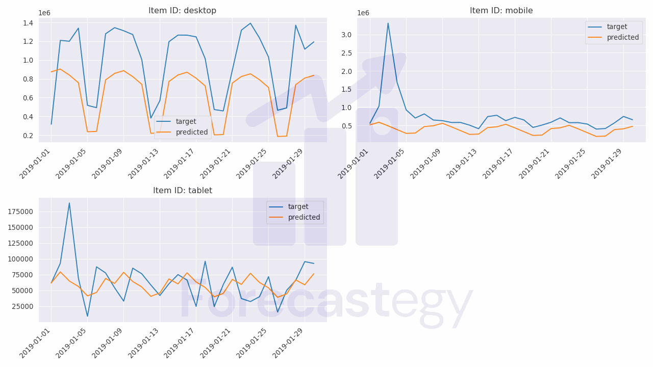
These are a few sample predictions from the model, displaying item_id, timestamp, the predicted mean values, and the true target values.
| item_id | timestamp | mean | target |
|---|---|---|---|
| desktop | 2019-01-01 00:00:00 | 874201 | 315674 |
| desktop | 2019-01-02 00:00:00 | 903386 | 1.20916e+06 |
| desktop | 2019-01-03 00:00:00 | 840079 | 1.19998e+06 |
| desktop | 2019-01-04 00:00:00 | 757855 | 1.33997e+06 |
| desktop | 2019-01-05 00:00:00 | 235723 | 516879 |
So, for example, the model predicted that the desktop time series would have 874,201 sessions on 2019-01-01, while the true value was 315,674 sessions.
Next, we evaluate the model’s performance in our external validation dataset using the same metric we chose during training:
mean_absolute_percentage_error(merged_df['target'], merged_df['mean'])
By calling this function from the sklearn.metrics module, we calculate the Mean Absolute Percentage Error (MAPE) between the true target values (original Sessions) and the mean forecasted values generated by our model.
This gives us a measure of our model’s performance in terms of forecasting accuracy.
AutoGluon automatically saves the fitted TimeSeriesPredictor object in a directory named 'AutogluonModels' (if you didn’t specify anything else in the path parameter).
If you want to load the saved model later, you simply need to specify the saved path and call the load() method:
saved_path = os.path.join('AutogluonModels', 'ag-20230422_173857')
predictor = TimeSeriesPredictor.load(saved_path)
In my case, the models were saved inside the ag-20230422_173857 directory.
Look for a learner.pkl file inside the directory and you’ll find the saved predictor object.
This process allows you to reuse the model without retraining, saving time and computational resources.
At the moment of writing, AutoGluon didn’t refit the models using the full data after doing the optimization.
Although you may see it done all the time on Kaggle, usually I don’t retrain ensembles using all the data in practice because it may cause instability and get different scores that what you got during the evaluation.
A Note For Windows Users
When I tried to run the code on Windows, I encountered an “access denied” error when trying to fit the DeepAR model.
I couldn’t solve it, so I rented a cloud GPU instance and ran the code on Linux.
You can do it or just ignore the DeepAR model in your ensemble.