In this article you will learn an easy, fast, step-by-step way to use Convolutional Neural Networks for multiple time series forecasting in Python.
We will use the NeuralForecast library which implements the Temporal Convolutional Network (TCN) architecture.
Temporal Convolutional Network (TCN)
This architecture is a variant of the Convolutional Neural Network (CNN) architecture that is specially designed for time series forecasting.
It was first presented as WaveNet.
 Source: WaveNet: A Generative Model for Raw Audio
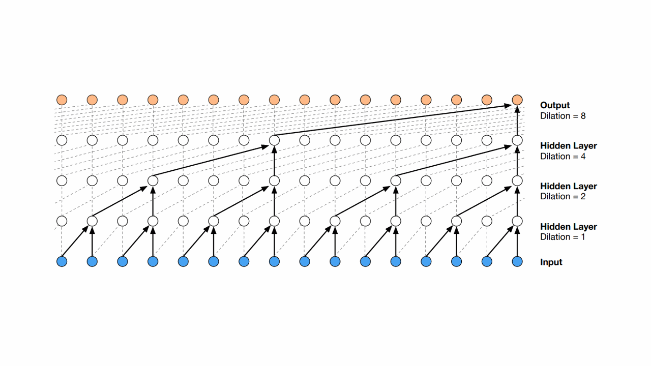
The main ingredient that makes it different from other convolutional networks is that it uses “causal and dilated convolutions.”
Causal convolutions force the model to learn the dependence between the steps without violating the natural order of time.
This is different from other convolutional networks that consider all available data in a sequence for modeling (before and after the current step).
The dilation technique helps it process an increasingly larger portion of the time series steps as it advances to the deeper layers.
In general, as you can see in the image, the dilation factor is doubled at each layer.
Unit 2 in the first hidden layer processes the information from steps 1 and 2.
Unit 4 in the second hidden layer processes steps 1, 2, 3, and 4 through the processing of hidden units 2 and 4 from the first hidden layer.
And so on.
These networks are generally faster to train than recurrent networks.
Let’s learn how you can use it in your time series forecasting projects.
How to Install NeuralForecast With and Without GPU Support
As NeuralForecast uses deep learning methods, if you have a GPU, it is important to have CUDA installed so that the models run faster.
To check if you have a GPU installed and correctly configured with PyTorch (backend library), run the code below:
import torch
print(torch.cuda.is_available())
This function returns True if you have a GPU installed and correctly configured, and False otherwise.
If you have a GPU but do not have PyTorch installed with it enabled, check the PyTorch official website for instructions on how to install the correct version.
I recommend that you install PyTorch first!!
The command I used to install PyTorch with GPU enabled was:
conda install pytorch pytorch-cuda=11.7 -c pytorch -c nvidia
If you don’t have a GPU, don’t worry, the library still works fine, it just won’t be as fast.
Installing it is very simple, just run the command below:
pip install neuralforecast
or if you use Anaconda:
conda install -c conda-forge neuralforecast
How To Prepare Time Series Data For The Temporal Convolutional Network
We will use real sales data from the Favorita store chain, from Ecuador.
We have sales data from 2013 to 2017 for multiple stores and product categories.
To measure the model’s performance, we will use WMAPE (Weighted Mean Absolute Percentage Error) with the absolutes of the actual values as weights.
import pandas as pd
import numpy as np

def wmape(y_true, y_pred):
    return np.abs(y_true - y_pred).sum() / np.abs(y_true).sum()
This is an adapted version of MAPE (Mean Absolute Percentage Error) that solves the problem of division by zero when there are no sales for a specific day.
For this tutorial I will use only the data from one store and two product categories.
You can use as many categories, SKUs, stores, etc as you want.
path = 'train.csv'
data = pd.read_csv(path, index_col='id', parse_dates=['date'])

data2 = data.loc[(data['store_nbr'] == 1) & (data['family'].isin(['MEATS', 'PERSONAL CARE'])), ['date', 'family', 'sales', 'onpromotion']]
This data doesn’t contain a record for December 25, so I just copied the sales from December 18 to December 25 to keep the weekly pattern.
dec25 = list()
for year in range(2013,2017):
    for family in ['MEATS', 'PERSONAL CARE']:
        dec18 = data2.loc[(data2['date'] == f'{year}-12-18') & (data2['family'] == family)]
        dec25 += [{'date': pd.Timestamp(f'{year}-12-25'), 'family': family, 'sales': dec18['sales'].values[0], 'onpromotion': dec18['onpromotion'].values[0]}]
data2 = pd.concat([data2, pd.DataFrame(dec25)], ignore_index=True).sort_values('date')
The columns are:
date: date of the recordfamily: product categorysales: sales amountonpromotion: how many products of that category were on promotion on that day
weekday = pd.get_dummies(data2['date'].dt.weekday)
weekday.columns = ['weekday_' + str(i) for i in range(weekday.shape[1])]

data2 = pd.concat([data2, weekday], axis=1)
Let’s use the weekday as an additional feature.
It can be transformed as an ordinal or categorical variable, but here I will use the categorical approach which is more common.
In general, using additional information that is relevant to the problem can improve the model’s performance.
Date components like weekday, month, day of the month are important to capture seasonal patterns.
There are a ton of additional information that we could add, like temperature, rain, holidays, etc.
data2 = data2.rename(columns={'date': 'ds', 'sales': 'y', 'family': 'unique_id'})
This library expects the columns to be named in the following format:
ds: date of the recordy: target variable (sales amount)unique_id: unique identifier of the time series (product category)
unique_id should identify each time series you have.
If we had more than one store, we would have to add the store number along with the categories to unique_id.
An example would be unique_id = store_nbr + '_' + family.
This is the final version of our dataframe data2:
| ds | unique_id | y | onpromotion | weekday_0 | weekday_1 | weekday_2 | weekday_3 | weekday_4 | weekday_5 | weekday_6 |
|---|---|---|---|---|---|---|---|---|---|---|
| 2013-01-01 00:00:00 | MEATS | 0 | 0 | 0 | 1 | 0 | 0 | 0 | 0 | 0 |
| 2013-01-01 00:00:00 | PERSONAL CARE | 0 | 0 | 0 | 1 | 0 | 0 | 0 | 0 | 0 |
| 2013-01-02 00:00:00 | MEATS | 369.101 | 0 | 0 | 0 | 1 | 0 | 0 | 0 | 0 |
| 2013-01-02 00:00:00 | PERSONAL CARE | 194 | 0 | 0 | 0 | 1 | 0 | 0 | 0 | 0 |
| 2013-01-03 00:00:00 | MEATS | 272.319 | 0 | 0 | 0 | 0 | 1 | 0 | 0 | 0 |
A row for each record containing the date, the time series ID (family in our example), the target value and columns for external variables (onpromotion).
Notice the time series records are stacked on top of each other.
Let’s split the data into train and validation sets.
Time Series Validation Split
You should never use random or k-fold validation for time series.
That would cause data leakage, as you would be using future data to train your model.
In practice, you can’t take random samples from the future to train your model, so you can’t use them here.
To avoid this issue, we will use a simple time series split between past and future.
A career tip: knowing how to do time series validation correctly is a skill that will set you apart from many data scientists (even experienced ones!).
Our training set will be all the data between 2013 and 2016 and our validation set will be the first 3 months of 2017.
train = data2.loc[data2['ds'] < '2017-01-01']
valid = data2.loc[(data2['ds'] >= '2017-01-01') & (data2['ds'] < '2017-04-01')]
h = valid['ds'].nunique()
Temporal Convolutional Network Hyperparameters
The implementation of the TCN in this library uses an encoder-decoder architecture.
The goal is to use a TCN to learn an optimized numerical representation of past observations with the encoder and then send this representation to a simple feedforward neural network (decoder) to generate predictions.
There are several hyperparameters to tune and NeuralForecast gives us an object that will automatically search for the best combination based on an internal validation error.
Still, it is important to understand what they are and the default value ranges that the library uses to optimize them.
I recommend that you run the search using the default ranges, especially if you don’t have much experience with neural networks.
The numbers shown here as default options are not necessarily the only possible ones, but just intervals chosen by the library’s creator as sensible to optimize.
kernel_size
This is the size of each filter used in the TCN convolution layers.
A filter is simply a weight vector that slides over the time series to generate a new sequence of values.
We can think of this new sequence as a simple transformation of the time series.
If we have a time series with 10 observations and a filter with a size of 2, first we multiply its two weights by the first two values of the time series and add the result.
This gives us the value of the first element of the transformed sequence.
In the second step, we multiply the same two weights by values 2 and 3 of the time series and add the result to get the second element of the transformed sequence.
And so it goes until the last.
We apply several different filters to generate several transformed sequences.
The idea is that these transformations better represent the patterns that we need to predict the next observations.
It differs from a regular feedforward neural network, as the latter uses only one set of weights to transform the inputs in each layer.
This hyperparameter is not optimized during the automatic search and receives the default value of 2, like in the original TCN diagram.
dilations
This is the value of the dilation interval of the filters: how many time units they should skip when applying the transformation.
They are also fixed values, multiples of 2, as per the diagram above.
input_size_multiplier
The first value optimized during the automatic search.
It defines the number of steps of the time series that will be used as input for the TCN (input features).
The possible values are -1, 4, 16, and 64.
But be careful, this value is multiplied by the horizon!
That is, a value equal to 4 means the input will be 4 times the horizon (4 * 90 = 360 days in our example).
If the value is -1, the network will use all past steps as input.
encoder_hidden_size
This is the size of the encoded representation outputted by the TCN, which is also the number of filters applied.
The number of units in this representation directly affects the network’s ability to learn complex patterns.
The larger, the more complex the patterns it can learn, but it has a higher risk of overfitting.
This hyperparameter is optimized during the automatic search. Its possible values are 10, 20, 40 and 80.
context_size
After the TCN emits its outputs, they are transformed again to represent the overall context of the time series information.
We can think of this as a summary of the most important information that we need to make predictions for the next steps.
It is a vector of size defined by context_size.
Possible values for this hyperparameter are 5, 10, and 50.
decoder_hidden_size
This is the number of units in the hidden layers of the feedforward neural network that acts as the decoder.
It has two hidden layers by default, and this is the number of units in each of them, not the total between them.
Two values are tested during the search: 64 and 128.
learning_rate
One of the most impactful hyperparameters, it defines how much each optimization step will modify the network weights.
The lower the learning_rate, the slower the optimization, but also makes it more stable.
During tuning, a value is sampled from a log uniform distribution and can range from 0.0001 to 0.1.
max_steps
The maximum number of times the neural network will update its weights during training.
It is closely tied and inversely proportional to the learning_rate.
Two values are tested: 500 and 1000.
Training a Temporal Convolutional Network In Python
It’s time to start the hyperparameter tuning search.
from neuralforecast import NeuralForecast
from neuralforecast.auto import AutoTCN

models = [AutoTCN(h=h,
                   num_samples=30,
                   loss=WMAPE())]

model = NeuralForecast(models=models, freq='D')
model.fit(train)
First we create a list with a single AutoTCN object and pass it to NeuralForecast.
The library allows us to train several models in the same object, but because this is a tutorial, we will only use TCN.
AutoTCN takes the following arguments:
h: the forecast horizon (how many steps into the future we want to predict)num_samples: the number of hyperparameter combinations that will be tested during the hyperparameter tuning. By default, the search is random.loss: the loss function to optimize during training. I am using a custom PyTorch WMAPE loss.
In practice, testing 30 combinations finds a good solution in a reasonable amount of time.
In the NeuralForecast object, we pass the argument freq that informs the frequency of the time series. In our case, it’s daily.
Then we just call the fit method and pass the training data to start training the model.
p = model.predict().reset_index()
p = p.merge(valid[['ds','unique_id', 'y']], on=['ds', 'unique_id'], how='left')
Now that we have a trained model, we can use it to make predictions by calling the predict method.
I merged the predictions with the validation data to make it easier to calculate the error metrics.
This is what the predictions dataframe looks like:
| unique_id | ds | AutoTCN | y |
|---|---|---|---|
| MEATS | 2017-01-01 00:00:00 | 122.66 | 0 |
| PERSONAL CARE | 2017-01-01 00:00:00 | 101.177 | 0 |
| PERSONAL CARE | 2017-01-02 00:00:00 | 150.795 | 81 |
| MEATS | 2017-01-02 00:00:00 | 242.997 | 116.724 |
| MEATS | 2017-01-03 00:00:00 | 247.094 | 344.583 |
Now let’s plot the predictions and the actual values to do a visual inspection.
fig, ax = plt.subplots(2, 1, figsize = (1280/96, 720/96))
fig.tight_layout(pad=7.0)
for ax_i, unique_id in enumerate(['MEATS', 'PERSONAL CARE']):
    plot_df = pd.concat([train.loc[train['unique_id'] == unique_id].tail(30),
                         p.loc[p['unique_id'] == unique_id]]).set_index('ds') # Concatenate the train and forecast dataframes
    plot_df[['y', 'AutoTCN']].plot(ax=ax[ax_i], linewidth=2, title=unique_id)


    ax[ax_i].grid()

print(wmape(p['y'], p['AutoTCN']))
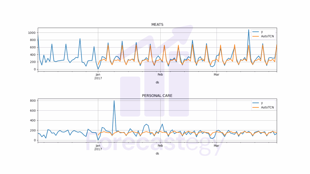
This model has a WMAPE of 20.49%.
We can see the combinations of hyperparameters that were tested during the search by calling the get_dataframe method.
results_df = models[0].results.get_dataframe().sort_values('loss')
results_df
| loss | config/encoder_hidden_size | config/decoder_hidden_size | config/max_steps |
|---|---|---|---|
| 0.598952 | 50 | 128 | 500 |
| 0.600814 | 50 | 64 | 1000 |
| 0.600958 | 100 | 128 | 1000 |
| 0.601555 | 100 | 128 | 500 |
| 0.602398 | 100 | 128 | 1000 |
It returns a DataFrame with the loss value and the hyperparameters tested for each combination.
This is very useful to understand which hyperparameters are more important for the model and guide your next steps.
To get the best hyperparameters, we call the get_best_result method.
best_config = models[0].results.get_best_result().metrics['config']
best_config

{'h': 90,
 'encoder_hidden_size': 50,
 'context_size': 50,
 'decoder_hidden_size': 128,
 'learning_rate': 0.00026729929225440886,
 'max_steps': 500,
 'batch_size': 16,
 'loss': WMAPE(),
 'check_val_every_n_epoch': 100,
 'random_seed': 18,
 'input_size': 5760}
Let’s use these hyperparameters to train a new model using external variables and see if we can improve the results.
Training a Temporal Convolutional Network with External Variables in Python
Here is the full code to train a TCN model with external variables.
from neuralforecast import NeuralForecast
from neuralforecast.models import TCN

models = [TCN(scaler_type='standard',
        futr_exog_list=['onpromotion', 'weekday_0',
       'weekday_1', 'weekday_2', 'weekday_3', 'weekday_4', 'weekday_5',
       'weekday_6'],
               **best_config)]

model = NeuralForecast(models=models, freq='D')
model.fit(train)

p = model.predict(futr_df=valid).reset_index()
p = p.merge(valid[['ds','unique_id', 'y']], on=['ds', 'unique_id'], how='left')

fig, ax = plt.subplots(2, 1, figsize = (1280/96, 720/96))
fig.tight_layout(pad=7.0)
for ax_i, unique_id in enumerate(['MEATS', 'PERSONAL CARE']):
    plot_df = pd.concat([train.loc[train['unique_id'] == unique_id].tail(30),
                         p.loc[p['unique_id'] == unique_id]]).set_index('ds')
    plot_df[['y', 'TCN']].plot(ax=ax[ax_i], linewidth=2, title=unique_id)

    ax[ax_i].grid()

print(wmape(p['y'], p['TCN']))
We need to make a few changes:
- Instead of
AutoTCN, we useTCNto instantiate the model. - We pass the
futr_exog_listargument to theTCNobject. This argument is a list of the names of the columns with external variables that we want to use in the model. - We pass a
scaler_type. Scaling the data usually improves model convergence, but this is not optimized byAutoTCN, so I tried it manually here. - We pass the
best_configdictionary as named arguments to theTCNobject. - In the
predictmethod, we pass thefutr_dfargument with the values for the external variables in the future time steps.
You have to think if the external variables will be available at the time of the forecast when you use this model in production.
If it’s a variable like temperature, you need to replace the true historical values with an estimate in the same way you will do when deployed.
Using data for the external variables that is available only in the historical data but not in production is a subtle mistake that will lead to overoptimistic results.
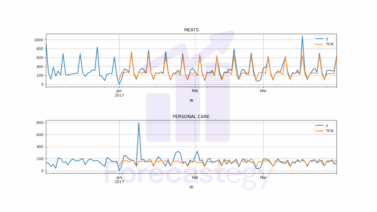
I tried the two scalers available and using none, and these were the results:
- No scaler: 19.72%
- Standard scaler: 19.46%
- Robust scaler: 19.63%
The results were very similar, most of it comes from using the external variables and not the scaler.
As it costs us almost nothing to use the scaler, I would recommend using it.
Now that you have a CNN, try to improve the solution by building an ensemble of models.