
Imagine having a robust forecasting solution capable of handling multiple time series data without relying on complex feature engineering.
That’s where N-BEATS comes in!
In this tutorial, I’ll break down its inner workings, walk you through the process of installing and configuring NeuralForecast to train an N-BEATS model in Python, and show you how to effectively prepare and split your time series data.
Furthermore, we’ll explore hyperparameter tuning with Optuna.
By the time you finish this tutorial, you’ll be well-prepared to leverage N-BEATS in your forecasting projects.
Let’s dive in!
What Is N-BEATS?
N-BEATS is a cutting-edge deep learning architecture designed specifically for time-series forecasting.
It’s one of the most successful non-recurrent neural network architectures for time-series forecasting.
With it, you can forecast multiple time-series data without relying on time-series-specific feature engineering.
Which makes it an excellent choice for tackling a wide range of forecasting problems.
At its core, N-BEATS comprises a series of basic building blocks.
Each block receives an input and produces two outputs: a forward forecast and a backcast, which represents the block’s best estimate of the input.
The full architecture is created by stacking these blocks together in a hierarchical structure.
How Does N-BEATS Work? (Architecture Overview)
 source:https://nixtla.github.io/neuralforecast/imgs_models/nbeats.png
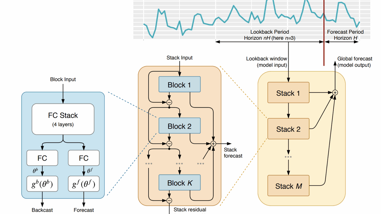
Basic Building Blocks
These blocks have two fully connected layers in a fork architecture after a stack of fully connected layers.
Once the initial stack of layers has processed the input data, the subsequent forecast and backcast layers come into play.
These layers use the forward and backward expansion coefficients generated by the initial fully connected network to create the final forecast and backcast outputs.
The forecast layers focus on generating accurate predictions for future data points, while the backcast layers work on estimating the input values themselves, given the constraints on the functional space that the network can use to approximate signals.
Stacking Blocks
These basic building blocks are stacked together using a technique known as “doubly residual stacking.”
This method creates a hierarchical structure with residual connections across different layers, allowing for better interpretability and a more transparent network structure.
Each block receives an input and generates a forecast (forward prediction) and a backcast (backward estimation).
The backcast output of the previous block is subtracted from its input to create the input for the next block.
This residual branch plays a key role in how the network processes the input signal.
By handling the input signal step-by-step, it ensures that each block focuses on a specific part of the data, making the overall prediction more accurate and efficient.
It kinda reminds me of boosting ensembles.
The partial forecasts, created by individual blocks, each capture different patterns and components of the input data.
As we move through the hierarchical structure, these partial forecasts are combined to form the final output.
This creates a hierarchical decomposition of the forecasting process, where forecasts from the basic building blocks are combined to form the overall prediction.
Now that you have a basic understanding of how N-BEATS works, let’s see how to use it in Python.
How to Install NeuralForecast With and Without GPU Support
As NeuralForecast uses deep learning methods, if you have a GPU, it is important to have CUDA installed so that the models run faster.
To check if you have a GPU installed and correctly configured with PyTorch (backend library), run the code below:
import torch
print(torch.cuda.is_available())
This function returns True if you have a GPU installed and correctly configured, and False otherwise.
If you have a GPU but do not have PyTorch installed with it enabled, check the PyTorch official website for instructions on how to install the correct version.
I recommend that you install PyTorch first!!
The command I used to install PyTorch with GPU enabled was:
conda install pytorch pytorch-cuda=11.8 -c pytorch -c nvidia
If you don’t have a GPU, don’t worry, the library still works fine, it just won’t be as fast.
Installing it is very simple, just run the command below:
pip install neuralforecast
or if you use Anaconda:
conda install -c conda-forge neuralforecast
How To Prepare Time Series Data For N-BEATS In Python
Let’s use the very practical example of sales forecasting in this tutorial.
We will use real sales data from the Favorita store chain, from Ecuador.
We have sales data from 2013 to 2017 for multiple stores and product categories.
For this tutorial I will use only the data from one store and two product categories.
You can use as many categories, SKUs, stores, etc as you want.
import pandas as pd
import numpy as np

path = 'train.csv'
data = pd.read_csv(path, index_col='id', parse_dates=['date'])

data2 = data.loc[(data['store_nbr'] == 1) & (data['family'].isin(['MEATS', 'PERSONAL CARE'])), ['date', 'family', 'sales', 'onpromotion']]
This data doesn’t contain a record for December 25, so I just copied the sales from December 18 to December 25 to keep the weekly pattern.
dec25 = list()
for year in range(2013,2017):
    for family in ['MEATS', 'PERSONAL CARE']:
        dec18 = data2.loc[(data2['date'] == f'{year}-12-18') & (data2['family'] == family)]
        dec25 += [{'date': pd.Timestamp(f'{year}-12-25'), 'family': family, 'sales': dec18['sales'].values[0], 'onpromotion': dec18['onpromotion'].values[0]}]
data2 = pd.concat([data2, pd.DataFrame(dec25)], ignore_index=True).sort_values('date')
The columns are:
date: date of the recordfamily: product categorysales: sales amountonpromotion: how many products of that category were on promotion on that day
In general, using additional information that is relevant to the problem can improve the model’s performance.
There are a ton of additional information that we could add, like temperature, rain, holidays, etc.
data2 = data2.rename(columns={'date': 'ds', 'sales': 'y', 'family': 'unique_id'})
This library expects the columns to be named in the following format:
ds: date of the recordy: target variable (sales amount)unique_id: unique identifier of the time series (product category)
unique_id should identify each time series you have.
If we had more than one store, we would have to add the store number along with the categories to unique_id.
An example would be unique_id = store_nbr + '_' + family.
This is the final version of our dataframe data2:
| ds | unique_id | y | onpromotion |
|---|---|---|---|
| 2013-01-01 00:00:00 | MEATS | 0 | 0 |
| 2013-01-01 00:00:00 | PERSONAL CARE | 0 | 0 |
| 2013-01-02 00:00:00 | MEATS | 369.101 | 0 |
| 2013-01-02 00:00:00 | PERSONAL CARE | 194 | 0 |
| 2013-01-03 00:00:00 | MEATS | 272.319 | 0 |
A row for each record containing the date, the time series ID (family in our example), the target value and columns for external variables (onpromotion).
Notice the time series records are stacked on top of each other.
Let’s split the data into train and validation sets.
How To Split Time Series Data For Validation
You should never use random or k-fold validation for time series.
That would cause data leakage, as you would be using future data to train your model.
In practice, you can’t take random samples from the future to train your model, so you can’t use them here.
To avoid this issue, we will use a simple time series split between past and future.
A career tip: knowing how to do time series validation correctly is a skill that will set you apart from many data scientists (even experienced ones!).
Our training set will be all the data between 2013 and 2016 and our validation set will be the first 3 months of 2017.
train = data2.loc[data2['ds'] < '2017-01-01']
valid = data2.loc[(data2['ds'] >= '2017-01-01') & (data2['ds'] < '2017-04-01')]
h = valid['ds'].nunique()
How To Train N-BEATS In Python With NeuralForecast
Let’s train a vanilla model first, with the default hyperparameters to understand the main code and then we will explore and tune the hyperparameters.
from neuralforecast import NeuralForecast
from neuralforecast.models import NBEATS
from neuralforecast.losses.pytorch import DistributionLoss

models = [NBEATS(h=h,input_size=7,
                 loss=DistributionLoss(distribution='Poisson', level=[90]),
                 max_steps=100,
                 scaler_type='standard',
               futr_exog_list=['onpromotion'])]

model = NeuralForecast(models=models, freq='D')
model.fit(train)

p =  model.predict(futr_df=valid).reset_index()
p = p.merge(valid[['ds','unique_id', 'y']], on=['ds', 'unique_id'], how='left')
Here, we create an instance of the NBEATS class, passing the following arguments:
h: horizon, the number of steps into the future we want to predictloss: the loss function that will be used to optimize the weights of the networkfutr_exog_list: a list of the names of the external variables we want to use in the forecastinput_size: the number of past time steps the model will use to predict the nexthsteps
In this case I picked the DistributionLoss class, which implements the very successful loss function used in DeepAR.
You can play with the distribution and the confidence level to adjust the loss function to your needs.
Here I am using a Poisson distribution with a 90% confidence interval (5% on each side).
There are three types of external variables we can use with this implementation:
futr_exog_list: external variables that are available for the forecast horizon. In this examples, I am assuming we know the days in the future when we will run promotions.hist_exog_list: external variables that are available only for the historical data. For example, if we wanted to adjust for promotions during training, but didn’t know the days when we would have promotions in the future.stat_exog_list: If you have static external variables (for example, the store’s city), you can use this. It will automatically add the variables to the input for the forecast horizon.
Lastly, we pass the list of models to the NeuralForecast class and set the data frequency as D (daily).
model.fit(train)

p =  model.predict(futr_df=valid).reset_index()
p = p.merge(valid[['ds','unique_id', 'y']], on=['ds', 'unique_id'], how='left')
We use the fit method to train the model, passing a DataFrame to futr_df with the additional columns for the forecast horizon.
If you didn’t use any external variables, you don’t need to pass anything.
The predict method returns a DataFrame with the predictions for the horizon h, starting from one period after the last date in the training set.
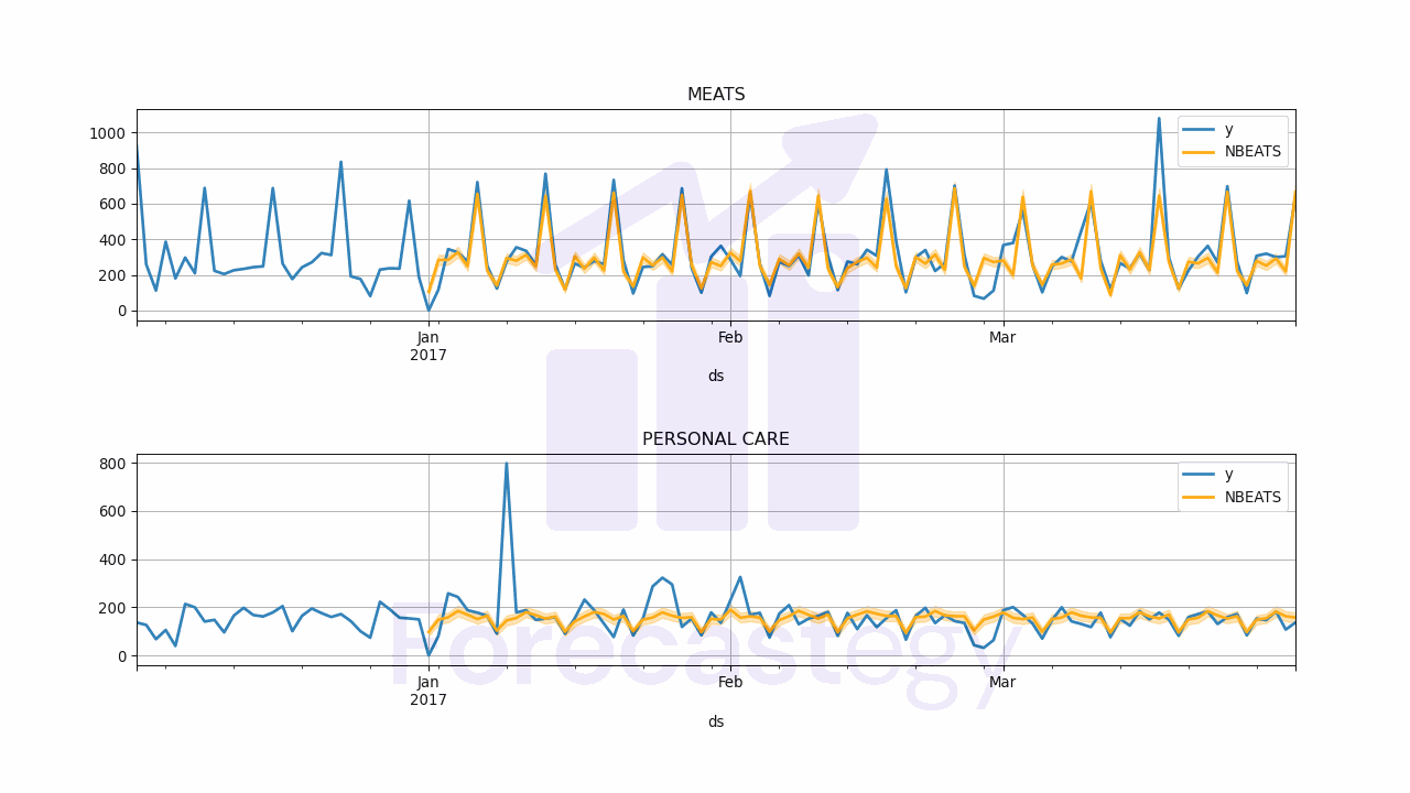
In order to evaluate the performance of the model I merged the targets with the predictions.
This is what p looks like:
| unique_id | ds | NBEATS | NBEATS-median | NBEATS-lo-90 | NBEATS-hi-90 | y |
|---|---|---|---|---|---|---|
| MEATS | 2017-01-01 00:00:00 | 151.376 | 151.5 | 131 | 173 | 0 |
| MEATS | 2017-01-02 00:00:00 | 214.225 | 214 | 189 | 240 | 116.724 |
| MEATS | 2017-01-03 00:00:00 | 201.957 | 202 | 179 | 224 | 344.583 |
| MEATS | 2017-01-04 00:00:00 | 237.627 | 237 | 213 | 265 | 326.203 |
| MEATS | 2017-01-05 00:00:00 | 219.031 | 219 | 196 | 243 | 274.205 |
unique_id: the time series ID of that rowds: the date corresponding to the predictionNBEATS: the point forecast (mean of the predicted samples when usingDistributionLoss)NBEATS-median: the median of the predicted samplesNBEATS-lo-90: the 90% confidence interval lower boundNBEATS-hi-90: the 90% confidence interval upper bound
How To Tune The N-BEATS Hyperparameters
There are a lot of hyperparameters to tune, but don’t feel overwhelmed!
I love to use Bayesian optimization to tune the hyperparameters of my models, and this can be done very easily with Optuna.
You can install Optuna with pip:
pip install optuna
Or with conda:
conda install -c conda-forge optuna
This is not an excuse to not understand the hyperparameters, but it can help you get started.
First, we need to define the objective function that will be optimized.
The function takes a trial object as its input, which is used to suggest various hyperparameter values.
from sklearn.metrics import mean_absolute_error
import optuna

def objective(trial):
    input_size = trial.suggest_int('input_size', 1, 60)

    n_blocks_season = trial.suggest_int('n_blocks_season', 1, 3)
    n_blocks_trend = trial.suggest_int('n_blocks_trend', 1, 3)
    n_blocks_identity = trial.suggest_int('n_blocks_ident', 1, 3)

    mlp_units_n = trial.suggest_categorical('mlp_units', [32, 64, 128])
    num_hidden = trial.suggest_int('num_hidden', 1, 3)

    n_harmonics = trial.suggest_int('n_harmonics', 1, 5)
    n_polynomials = trial.suggest_int('n_polynomials', 1, 5)

    scaler_type = trial.suggest_categorical('scaler_type', ['standard', 'robust'])
    learning_rate = trial.suggest_loguniform('learning_rate', 1e-5, 1e-1)


    n_blocks = [n_blocks_season, n_blocks_trend, n_blocks_identity]
    mlp_units=[[mlp_units_n, mlp_units_n]]*num_hidden
    models = [NBEATS(h=h,input_size=input_size,
                 loss=DistributionLoss(distribution='Poisson', level=[90]),
                 max_steps=100,
                 futr_exog_list=['onpromotion'],
                 stack_types=['seasonality', 'trend', 'identity'],
                 mlp_units=mlp_units,
                 n_blocks=n_blocks,
                 learning_rate=learning_rate,
                 n_harmonics=n_harmonics,
                 n_polynomials=n_polynomials,
                 scaler_type=scaler_type)
                 ]
    model = NeuralForecast(models=models, freq='D')
    model.fit(train)

    p = model.predict(futr_df=valid).reset_index()
    p = p.merge(valid[['ds', 'unique_id', 'y']], on=['ds', 'unique_id'], how='left')

    loss = mean_absolute_error(p['y'], p['NBEATS'])

    return loss
In this function, we suggest the possible values for each hyperparameter using trial.suggest_* methods.
For example, suggest_int will pick an integer between the two values passed as arguments, suggest_categorical will pick one of the values passed as a list.
The ranges you see above are the ones I found to work well in practice, so they are a good starting point.
Here’s a breakdown of the hyperparameters, their influence on the model’s behavior and performance, and the rationale behind the chosen ranges:
input_size
input_size is an integer value representing the number of autoregressive inputs (lags) considered by the model.
In the context of time series forecasting, autoregressive inputs are one of the most effective ways to help the model capture the relationship between past and future values.
In this specific example, the input_size is set to a maximum of 60 to consider at most 2 months (60 days) of past data when making predictions.
It’s essential to adjust this value according to the frequency and characteristics of your data to ensure the model considers the appropriate amount of historical information when making forecasts.
n_blocks_*
n_blocks_* are three integer values (n_blocks_season, n_blocks_trend, and n_blocks_identity) that correspond to the number of blocks for each stack type (seasonality, trend, and identity) in the N-BEATS model.
Each block is a combination of a fully connected neural network layer and a type-specific operation (e.g., seasonality or trend).
The choice of the number of blocks for each stack type has a direct impact on the model’s capacity to capture the underlying patterns in your data.
For example, increasing the number of blocks for seasonality could provide the model with the ability to better capture complex seasonal patterns.
mlp_units_n and num_hidden
I find these arguments a bit confusing, so let me try to clarify it.
mlp_units_n determines the number of units, or nodes, in the hidden layers of the MLPs inside the blocks.
Each unit within a hidden layer is responsible for learning specific features or patterns in the input data.
Like many other hyperparameters, increasing the number of units can provide the model with the capacity to learn more complex patterns, but it may also increase the risk of overfitting.
num_hidden determines the total number of hidden layers in the MLP.
More hidden layers can allow the model to learn hierarchical representations, with each layer learning increasingly abstract features.
To configure the mlp_units argument, you need to pass a list of lists containing the number of hidden layers and their units.
Each outer list element corresponds to a layer in the MLPs, while each inner list element represents the number of hidden input and output units for that layer.
As a practical tip, setting the mlp_units_n to multiples of 2 can be beneficial, as GPUs often exhibit better performance with such configurations due to their architecture.
n_harmonics
n_harmonics is an integer value that specifies the number of harmonic terms for the seasonality stack type in the N-BEATS model.
Harmonic terms, in this context, are a way to model the periodic behavior in the data.
In simple terms, higher values can help capture more complex patterns within seasonal data.
However, setting this parameter too high can lead to overfitting, so it’s essential to find the right balance.
n_polynomials
n_polynomials is an integer value that denotes the polynomial degree for the trend stack type in the N-BEATS model.
The degree of the polynomial represents the highest power of the variable.
In the context of time series forecasting, higher polynomial degrees can capture more complex trends in the data.
Like with n_harmonics, finding the optimal value for this parameter is essential to avoid overfitting.
scaler_type
scaler_type is a categorical value that determines the type of scaler used for normalizing the temporal inputs in the N-BEATS model.
Normalizing, or scaling, the inputs can be an essential step in preparing your data for neural networks as it helps ensure that all features have the same magnitude, thus stabilizing the training process.
There are two choices available for scaler_type: ‘standard’ and ‘robust’.
The ‘standard’ scaler assumes that data scales it by removing the mean and dividing by the standard deviation.
The ‘robust’ scaler, on the other hand, is less influenced by outliers. It subtracts the median and divides by the median absolute deviation.
learning_rate
learning_rate is a floating-point value that represents the learning rate for the model’s optimization process.
The learning rate is an essential hyperparameter in training neural networks and other gradient-based optimization algorithms.
It controls the size of the steps the algorithm takes while updating the model’s parameters in search of the optimal weights.
When using a logarithmic scale, each step represents a multiplicative change, which enables the search to cover a broader range of values while still being able to hone in on specific regions.
This approach is particularly useful in discovering an optimal learning rate value for the model, as smaller learning rates can lead to more stable training and higher accuracy.
By using this scale, you increase the chances of identifying a learning rate that achieves a good balance between converging quickly and accurately on the optimal solution.
Running The Bayesian Optimization
To demonstrate, I set the loss to be the mean absolute error, but you can use any metric you want.
This is not the same loss function that will be used to train the model, it’s just a metric to evaluate the performance of the model on the validation set.
Finally, run the Optuna optimization:
study = optuna.create_study(direction='minimize')
study.optimize(objective, n_trials=30)
We set the direction to minimize because we want to minimize the loss function.
If this was a “positive is better” metric, like coverage probability, we would set it to maximize.
In practice, I find that 20 to 30 trials are enough to find a good set of hyperparameters.
After the optimization finishes, you can get the best set of hyperparameters with:
study.best_params
And the best value of the loss function (corresponding to the best hyperparameters) with:
study.best_value
Frequently Asked Questions
How To Train The N-BEATS With Multiple SKUs?
The only change is that your unique_id column will be the SKU. You can use the rest of the code as is.