So, you’ve already explored the world of LSTMs and now you’re curious about their sibling GRUs (Gated Recurrent Units) and how they can enhance your time series forecasting projects…
Great!
As machine learning practitioners, we’re always looking for ways to expand our knowledge and improve our model choices.
In this tutorial, we’ll take a deep dive into GRUs, covering their inner workings, and comparing them to LSTMs.
By the end of this tutorial, you’ll have a solid understanding of GRUs and be well-equipped to use them effectively in Python.
We will use the NeuralForecast library.
How GRUs Work In Simple Terms
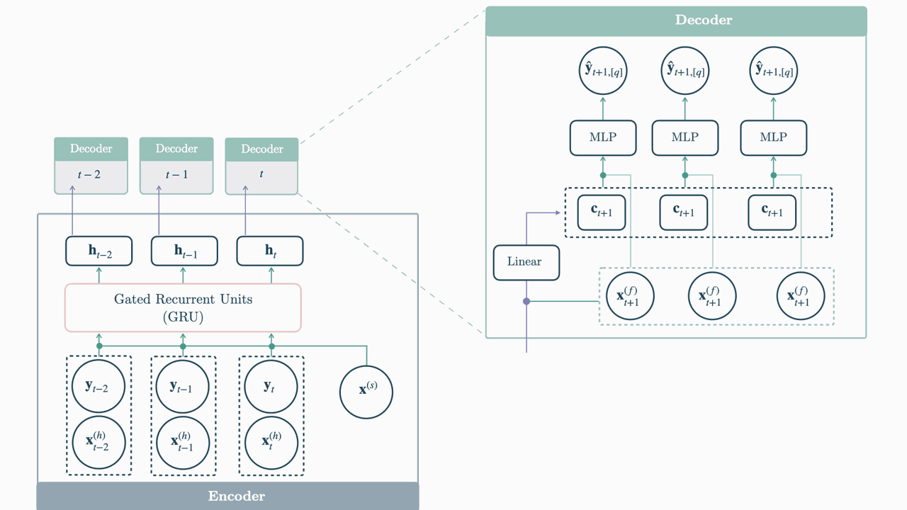
 source:https://nixtla.github.io/neuralforecast/imgs_models/gru.png
Let’s break down how a GRU works in simple terms.
GRUs are a type of recurrent neural network (RNN), which is designed to handle sequences of data, like time series or sentences.
The main feature of GRUs is their ability to “remember” past information while processing new data.
Imagine the GRU as a chef who needs to prepare a special dish (output) based on a recipe (sequence of data).
The chef has a mixing bowl, which represents the hidden state (memory).
Update Gate
Think of the update gate as the chef’s decision on the proportion of the current mixture in the bowl (previous memory) to retain, and the proportion of the new ingredients (new candidate state) to add.
If the update gate value is close to 1, it means the chef wants to use more of the current mixture, and less of the new ingredients.
If the update gate value is close to 0, the chef wants to use more new ingredients and less of the current mixture.
In this way, the update gate helps balance the old and new information when updating the overall memory.
At first, this was confusing to me, as I expected a higher update gate value to mean that the chef wants to use more of the new ingredients, but it was the contrary.
Reset gate
The reset gate represents the chef’s decision on how much of the current mixture to consider when preparing the new ingredients before they are added to the bowl.
If the reset gate value is close to 1, the chef wants to use the current mixture to influence how the new ingredients are prepared.
If the reset gate value is close to 0, the chef wants to disregard the current mixture and prepare the new ingredients independently.
This gate helps decide the influence of the past information on the preparation of the new candidate state.
These two gates work together to help the GRU decide what to remember and what to forget.
The gates are controlled by the data itself, allowing the GRU to learn and adapt to the sequence.
What Is The Difference Between GRUs And LSTMs
The main differences between GRUs and LSTMs are their structure, complexity, and performance.
Both are well-suited for time series forecasting, and the only way to find out which one is best for your data is to test them.
They have a particular architecture that allows them to remember information over time.
They achieve this by using “gates” – mechanisms that regulate the flow of information.
However, GRUs have two gates (update and reset), while LSTMs have three gates (input, output, and forget).
In simpler terms, you can think of gates as doors that allow or block the flow of information, helping the network decide what to remember or forget.
Since LSTMs have an extra gate, they’re generally more complex than GRUs.
This means that LSTMs may take longer to train, require more computational resources and are more prone to overfitting.
On the other hand, GRUs are simpler and faster to train. So, when choosing between the two, you might consider the available resources and time.
In some cases, LSTMs can outperform GRUs for certain tasks due to their additional gate.
However, this isn’t always true. Sometimes, GRUs perform just as well as LSTMs, especially with smaller datasets or when a simpler model is sufficient.
Like I said before, the only way to find out is to try both in your data.
How to Install NeuralForecast With and Without GPU Support
As NeuralForecast uses deep learning methods, if you have a GPU, it is important to have CUDA installed so that the models run faster.
To check if you have a GPU installed and correctly configured with PyTorch (backend library), run the code below:
import torch
print(torch.cuda.is_available())
This function returns True if you have a GPU installed and correctly configured, and False otherwise.
If you have a GPU but do not have PyTorch installed with it enabled, check the PyTorch official website for instructions on how to install the correct version.
I recommend that you install PyTorch first!!
The command I used to install PyTorch with GPU enabled was:
conda install pytorch pytorch-cuda=11.8 -c pytorch -c nvidia
If you don’t have a GPU, don’t worry, the library still works fine, it just won’t be as fast.
Installing it is very simple, just run the command below:
pip install neuralforecast
or if you use Anaconda:
conda install -c conda-forge neuralforecast
How To Prepare Time Series Data For The GRU
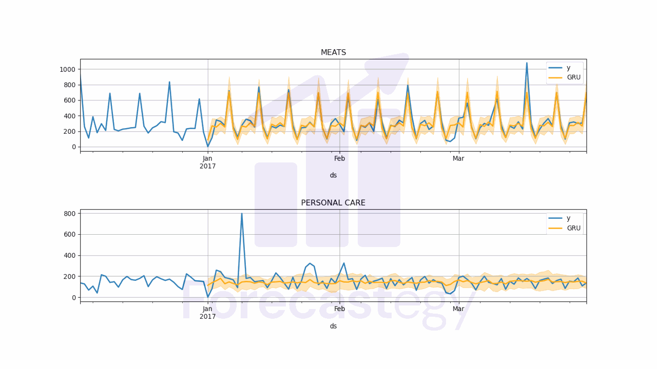
Let’s use the very practical example of sales forecasting) in this tutorial.
We will use real sales data from the Favorita store chain, from Ecuador.
We have sales data from 2013 to 2017 for multiple stores and product categories.
For this tutorial I will use only the data from one store and two product categories.
You can use as many categories, SKUs, stores, etc as you want.
import pandas as pd
import numpy as np

path = 'train.csv'
data = pd.read_csv(path, index_col='id', parse_dates=['date'])

data2 = data.loc[(data['store_nbr'] == 1) & (data['family'].isin(['MEATS', 'PERSONAL CARE'])), ['date', 'family', 'sales', 'onpromotion']]
This data doesn’t contain a record for December 25, so I just copied the sales from December 18 to December 25 to keep the weekly pattern.
dec25 = list()
for year in range(2013,2017):
    for family in ['MEATS', 'PERSONAL CARE']:
        dec18 = data2.loc[(data2['date'] == f'{year}-12-18') & (data2['family'] == family)]
        dec25 += [{'date': pd.Timestamp(f'{year}-12-25'), 'family': family, 'sales': dec18['sales'].values[0], 'onpromotion': dec18['onpromotion'].values[0]}]
data2 = pd.concat([data2, pd.DataFrame(dec25)], ignore_index=True).sort_values('date')
The columns are:
date: date of the recordfamily: product categorysales: sales amountonpromotion: how many products of that category were on promotion on that day
In general, using additional information that is relevant to the problem can improve the model’s performance.
There are a ton of additional information that we could add, like temperature, rain, holidays, etc.
data2 = data2.rename(columns={'date': 'ds', 'sales': 'y', 'family': 'unique_id'})
This library expects the columns to be named in the following format:
ds: date of the recordy: target variable (sales amount)unique_id: unique identifier of the time series (product category)
unique_id should identify each time series you have.
If we had more than one store, we would have to add the store number along with the categories to unique_id.
An example would be unique_id = store_nbr + '_' + family.
This is the final version of our dataframe data2:
| ds | unique_id | y | onpromotion |
|---|---|---|---|
| 2013-01-01 00:00:00 | MEATS | 0 | 0 |
| 2013-01-01 00:00:00 | PERSONAL CARE | 0 | 0 |
| 2013-01-02 00:00:00 | MEATS | 369.101 | 0 |
| 2013-01-02 00:00:00 | PERSONAL CARE | 194 | 0 |
| 2013-01-03 00:00:00 | MEATS | 272.319 | 0 |
A row for each record containing the date, the time series ID (family in our example), the target value and columns for external variables (onpromotion).
Notice the time series records are stacked on top of each other.
Let’s split the data into train and validation sets.
How To Split Time Series Data For Validation
You should never use random or k-fold validation for time series.
That would cause data leakage, as you would be using future data to train your model.
In practice, you can’t take random samples from the future to train your model, so you can’t use them here.
To avoid this issue, we will use a simple time series split between past and future.
A career tip: knowing how to do time series validation correctly is a skill that will set you apart from many data scientists (even experienced ones!).
Our training set will be all the data between 2013 and 2016 and our validation set will be the first 3 months of 2017.
train = data2.loc[data2['ds'] < '2017-01-01']
valid = data2.loc[(data2['ds'] >= '2017-01-01') & (data2['ds'] < '2017-04-01')]
h = valid['ds'].nunique()
What Is The Architecture Of NeuralForecast’s GRU?
This implementation uses an encoder and a decoder, a very successful architecture when dealing with sequential data.
The encoder will distill the input sequence into a compact representation, keeping the information that is important for the target we want to predict.
The decoder will receive these features (encoded representation) and make the predictions.
The encoder is a GRU cell and the decoder is a feedforward neural network (MLP).
There are a few hyperparameters that are important to know before training the model.
context_size
This parameter controls how many steps in the past will be used to predict the next step.
By default it is 10, which means that the network will use the last 10 steps to predict the next one.
The steps can be hours, days, weeks, etc, depending on the frequency of your data.
In our example, it’s daily data, so it will use the last 10 days to predict the next one.
encoder_hidden_size
Controls the number of units (neurons) of the encoder’s internal representation (hidden layer).
The larger it is, the more capacity the network has to learn complex patterns, but also increases the risk of overfitting.
All layers of the GRU will have the same number of units.
encoder_n_layers
Controls the number of layers in the encoder.
Just like the size of the internal representation, the larger the number of layers, the more capacity to learn complex patterns, but also more chances of overfitting.
encoder_dropout
This parameter controls the dropout rate of the encoder.
Dropout is a very effective regularization technique that helps prevent overfitting by zeroing out a random percentage of the units in each layer during training.
decoder_hidden_size
Controls the number of units (neurons) of the decoder’s internal representations.
The decoder is a regular feed-forward neural network (MLP).
decoder_layers
Controls the number of layers in the MLP decoder. It’s 2 by default.
scaler_type
Neural networks are very sensitive to the scale of the input data, so it’s usually a good idea to scale it.
The library has three options for scaling the data:
None: no scalingstandard: standard scalingrobust: robust scaling
standard scales the data by subtracting the mean and dividing by the standard deviation.
robust does it by subtracting the median and dividing by the mean absolute deviation.
learning_rate
One of the most important hyperparameters for any neural network.
It controls the step size used by the optimization algorithm to update the network’s weights.
If it’s too large, the algorithm may diverge and never find a good solution.
If it’s too small, the algorithm may take a long time to converge.
max_steps
This argument controls the maximum number of training steps.
It determines how many times the optimization algorithm will update the network’s weights.
The lower the learning_rate, the more steps are necessary for convergence.
Solutions with a high number of steps and a low learning_rate take longer to train, but tend to be more stable and performant.
How To Train GRU In Python
from neuralforecast import NeuralForecast
from neuralforecast.models import GRU
from neuralforecast.losses.pytorch import DistributionLoss

models = [GRU(h=h,
               loss=DistributionLoss(distribution='Normal', level=[90]),
               max_steps=100,
               encoder_n_layers=2,
               encoder_hidden_size=200,
               context_size=10,
               encoder_dropout=0.5,
               decoder_hidden_size=200,
               decoder_layers=2,
               learning_rate=1e-3,
               scaler_type='standard',
               futr_exog_list=['onpromotion'])]

model = NeuralForecast(models=models, freq='D')
model.fit(train)
We need the NeuralForecast and GRU classes to train the network.
NeuralForecast is an utility class to manage the internals of training the neural network.
GRU is the class that implements the architecture we saw above.
First we create a list with the models we want to train, in this case only GRU.
NeuralForecast was made to train multiple deep learning models at the same time, this is why we need to pass a list, even if it has only one model.
The GRU class has many arguments, including the hyperparameters I explained above.
Beyond them, you need to know:
h: horizon, the number of steps into the future we want to predictloss: the loss function that will be used to optimize the weights of the networkfutr_exog_list: a list of the names of the external variables we want to use in the forecast
In this case I picked the DistributionLoss class, which implements the very successful loss function used in DeepAR.
You can play with the distribution and the confidence level to adjust the loss function to your needs.
Here I am using a normal distribution with a 90% confidence interval (5% on each side).
There are three types of external variables we can use with this implementation:
futr_exog_list: external variables that are available for the forecast horizon. In this examples, I am assuming we know the days in the future when we will run promotions.hist_exog_list: external variables that are available only for the historical data. For example, if we wanted to adjust for promotions during training, but didn’t know the days when we would have promotions in the future.stat_exog_list: If you have static external variables (for example, the store’s city), you can use this. It will automatically add the variables to the input for the forecast horizon.
Lastly, we pass the list of models to the NeuralForecast class and set the data frequency as D (daily).
model.fit(train)

p =  model.predict(futr_df=valid).reset_index()
p = p.merge(valid[['ds','unique_id', 'y']], on=['ds', 'unique_id'], how='left')
We use the fit method to train the model, passing a DataFrame to futr_df with the additional columns for the forecast horizon.
If you didn’t use any external variables, you don’t need to pass anything.
The predict method returns a DataFrame with the predictions for the horizon h, starting from one period after the last date in the training set.
In order to evaluate the performance of the model I merged the targets with the predictions.
This is what p looks like:
| unique_id | ds | GRU | GRU-median | GRU-lo-90 | GRU-hi-90 | y |
|---|---|---|---|---|---|---|
| MEATS | 2017-01-01 00:00:00 | 92.2766 | 91.3605 | 23.3603 | 160.243 | 0 |
| MEATS | 2017-01-02 00:00:00 | 270.821 | 270.283 | 174.35 | 365.669 | 116.724 |
| MEATS | 2017-01-03 00:00:00 | 256.673 | 255.253 | 153.818 | 363.122 | 344.583 |
| MEATS | 2017-01-04 00:00:00 | 307.162 | 304.154 | 217.014 | 397.263 | 326.203 |
| MEATS | 2017-01-05 00:00:00 | 255.018 | 255.126 | 166.806 | 350.767 | 274.205 |
unique_id: the time series ID of that rowds: the date corresponding to the predictionGRU: the point forecast (mean of the predicted samples when usingDistributionLoss)GRU-median: the median of the predicted samplesGRU-lo-90: the 90% confidence interval lower boundGRU-hi-90: the 90% confidence interval upper bound
How To Tune The GRU Hyperparameters
If you feel overwhelmed by the number of hyperparameters, don’t worry, you are not alone.
I love to use Bayesian optimization to tune the hyperparameters of my models, and this can be done very easily with Optuna.
You can install Optuna with pip:
pip install optuna
Or with conda:
conda install -c conda-forge optuna
This is not an excuse to not understand the hyperparameters, but it can help you get started.
First, we need to define the objective function that will be optimized.
from sklearn.metrics import mean_absolute_error
import optuna

def objective(trial):
    encoder_n_layers = trial.suggest_int('encoder_n_layers', 1, 3)
    encoder_hidden_size = trial.suggest_categorical('encoder_hidden_size', [64, 128, 256])
    decoder_layers = trial.suggest_int('decoder_layers', 1, 3)
    encoder_dropout = trial.suggest_uniform('encoder_dropout', 0, 0.9)
    decoder_hidden_size = trial.suggest_categorical('decoder_hidden_size', [64, 128, 256])
    learning_rate = trial.suggest_loguniform('learning_rate', 1e-5, 1e-1)
    context_size = trial.suggest_int('context_size', 1, 60)
    scaler_type = trial.suggest_categorical('scaler_type', ['standard', 'robust'])

    models = [GRU(h=h,
                   loss=DistributionLoss(distribution='Normal', level=[90]),
                   max_steps=100,
                   encoder_n_layers=encoder_n_layers,
                   encoder_hidden_size=encoder_hidden_size,
                   context_size=context_size,
                   encoder_dropout=encoder_dropout,
                   decoder_hidden_size=decoder_hidden_size,
                   decoder_layers=decoder_layers,
                   learning_rate=learning_rate,
                   scaler_type=scaler_type,
                   futr_exog_list=['onpromotion'])]

    model = NeuralForecast(models=models, freq='D')
    model.fit(train)

    p = model.predict(futr_df=valid).reset_index()
    p = p.merge(valid[['ds', 'unique_id', 'y']], on=['ds', 'unique_id'], how='left')

    loss = mean_absolute_error(p['y'], p['GRU'])

    return loss
In this function, we suggest the possible values for each hyperparameter using trial.suggest_* methods.
For example, suggest_int will pick an integer between the two values passed as arguments, suggest_categorical will pick one of the values passed as a list.
The ranges you see above are the ones I found to work well in practice, so they are a good starting point.
I like to set the hidden_size to multiples of 2 because GPUs tend to work better with it.
I set the context_size to a maximum of 60 because I want it to consider at most 2 months (60 days). Remember to adjust it according to the frequency of your data.
To demonstrate, I set the loss to be the mean absolute error, but you can use any metric you want.
This is not the same loss function that will be used to train the model, it’s just a metric to evaluate the performance of the model on the validation set.
Finally, run the Optuna optimization:
study = optuna.create_study(direction='minimize')
study.optimize(objective, n_trials=30)
We set the direction to minimize because we want to minimize the loss function.
If this was a “positive is better” metric, like coverage probability, we would set it to maximize.
In practice, I find that 20 to 30 trials are enough to find a good set of hyperparameters.
After the optimization finishes, you can get the best set of hyperparameters with:
study.best_params
And the best value of the loss function (corresponding to the best hyperparameters) with:
study.best_value
Frequently Asked Questions
How To Train The GRU With Multiple SKUs?
The only change is that your unique_id column will be the SKU. You can use the rest of the code as is.