Today, we’re going to explore multiple time series forecasting with LightGBM in Python.
If you’re not already familiar, LightGBM is a powerful open-source gradient boosting framework that’s designed for efficiency and high performance.
It’s a great tool for tackling large datasets and can help you create accurate predictions in a flash.
When combined with the MLForecast library, it becomes a versatile and scalable solution for multiple time series forecasting.
Let’s dive into the step-by-step process of preparing our data, defining our LightGBM model, and training it using MLForecast in Python.
I will also cover some tips and tricks for optimizing the performance of our model, as well as how to evaluate its accuracy and make predictions for future time periods.
Let’s get started!
Installing LightGBM And MLForecast
It’s easy to install LightGBM and MLForecast using pip:
pip install lightgbm
pip install mlforecast
Preparing Time Series Data for LightGBM
We will use data from the City of Los Angeles website traffic dataset on Kaggle.
This dataset contains the number of user sessions for the City of Los Angeles website for each day from 2014 to 2019.
Sessions are periods of time when a user is active in a website.
Usually they are measured by looking at user activity and have a timeout after 30 minutes since the last user action.
For example, right now you are in a session on my website. If you leave the page and come back after 2 hours, you will be in a new session.
Let’s load the data and take a look at it:
import pandas as pd
import numpy as np
from matplotlib import pyplot as plt
import os

data = pd.read_csv(os.path.join(path, 'lacity.org-website-traffic.csv'),
                   parse_dates=['Date']).loc[:, ['Date', 'Device Category', 'Sessions']]
fixes = pd.DataFrame({'Date': pd.to_datetime(['2016-12-01', '2018-10-13']),
                      'Device Category': ['tablet', 'tablet'] ,
                      'Sessions': [np.nan, np.nan]})

data = pd.concat([data, fixes], axis=0, ignore_index=True)
data = data.rename(columns={'Device Category': 'unique_id', 'Sessions': 'y', 'Date': 'ds'})
data = data.sort_values(['unique_id', 'ds']).groupby('unique_id').apply(lambda x: x.fillna(method='ffill'))
| ds | unique_id | y |
|---|---|---|
| 2014-01-01 00:00:00 | desktop | 1032805 |
| 2014-01-01 00:00:00 | mobile | 537573 |
| 2014-01-01 00:00:00 | tablet | 92474 |
| 2014-01-02 00:00:00 | desktop | 2359710 |
| 2014-01-02 00:00:00 | mobile | 607544 |
We load the data with Pandas and take only 3 columns: the date, the device category, and the number of sessions.
The original data has more detailed information about the sessions, like the browser and number of visitors, but we don’t need it for this tutorial.
We then group the data by date and device category and sum the number of sessions for each group.
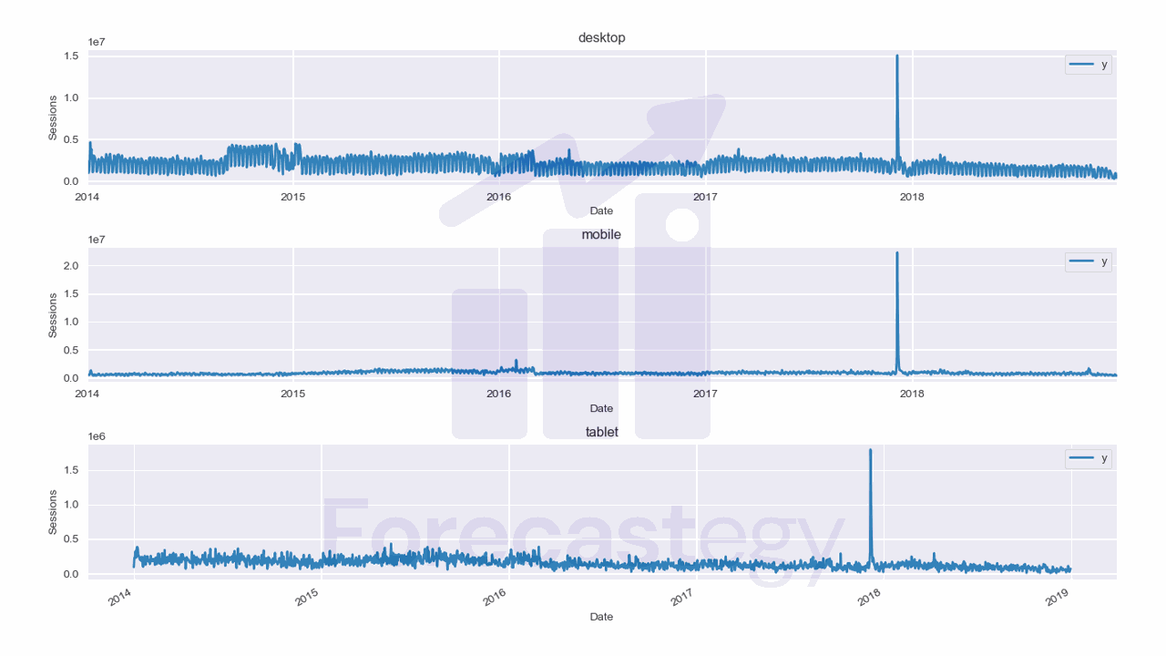
Here we have 3 time series: one for desktop, one for mobile, and one for tablet.
They are stacked in the long format, which means that each row represents a single observation.
This data has two points missing for the tablet device category, so we add them manually as np.nan, then fill with the previous day value.
Nixtla’s forecast libraries expect the data to have at least 3 columns: ds, unique_id, and y.
This doesn’t seem to be enforced in MLForecast, but it’s a good practice to follow.
ds is the date column, unique_id is the unique identifier for each time series, and y is the target variable.
In our case, each unique_id is a device category, but it can be an SKU, a store, a city or any other unique identifier of a time series.
Finally we split the data into train and test sets:
train = data.loc[data['ds'] < '2019-01-01']
valid = data.loc[(data['ds'] >= '2019-01-01') & (data['ds'] < '2019-04-01')]
h = valid['ds'].nunique()
I am using data from 2014 to 2018 as the training set and the first 3 months of 2019 as the validation set.
We set h to the number of days in the validation set. This is the horizon, or the number of steps we want to forecast.
This is what the training data looks like:

Training A LightGBM For Time Series Forecasting With MLForecast
MLForecast has a class that will handle most of the work for us.
from lightgbm import LGBMRegressor
from mlforecast import MLForecast

from window_ops.rolling import rolling_mean, rolling_max, rolling_min

models = [LGBMRegressor(random_state=0, n_estimators=100)]

model = MLForecast(models=models,
                   freq='D',
                   lags=[1,7,14],
                   lag_transforms={
                       1: [(rolling_mean, 7), (rolling_max, 7), (rolling_min, 7)],
                   },
                   date_features=['dayofweek', 'month'],
                   num_threads=6)


model.fit(train, id_col='unique_id', time_col='ds', target_col='y', static_features=[])

p = model.predict(horizon=h)
p = p.merge(valid[['unique_id', 'ds', 'y']], on=['unique_id', 'ds'], how='left')

from sklearn.metrics import mean_absolute_percentage_error
mean_absolute_percentage_error(p['y'], p['LGBMRegressor'])
We create a list with a single LightGBM model, then we create an instance of the MLForecast class.
This is the class that will handle the feature engineering and training of our model.
We can pass any of the usual hyperparameters of LightGBM to the constructor, like n_estimators and random_state, but we will use the default values for now.
We also pass the freq parameter, which is the frequency of the data. In our case, it’s daily data, so we set it to D.
The lags argument is a list of lags we want to use in our model. Lags are the number of steps in the past we want to use to predict the future.
So in our case, we are using the value of the target variable 1, 7, and 14 days before the timestamp date of the observation.
I explained the four basic features for time series forecasting in detail in the article about multiple time series forecasting with Scikit-learn.
This is why it’s important to have all dates, even the ones with missing values and zeros in the datasets, so these features can be computed correctly.
We also pass the lag_transforms argument, which is a dictionary with the lag as the key and a list of functions as the value.
These functions will be applied to the lagged series. For example, we are applying a rolling mean with a window of 7 days to the lag 1.
This means that we will have a feature that is the mean of the 7 last values of the target variable after shifting it 1 day.
You can pass any function that takes a NumPy array and returns a NumPy array. Use numba to speed up your functions, as recommended in the documentation.
I am using the window_ops library which is optimized and recommended by the developers of MLForecast.
Each tuple in the list of transforms is a function and its arguments. For example, the rolling_mean function takes a window size as its argument.
The best value for the window size is specific for each time series, so we need to try different values and see which one works best.
The date_features argument is a list of date components we want to extract from the date column.
These are important to help the model capture the seasonality of the data.
Finally, we pass the num_threads argument, which is the number of threads to use for parallel processing.
We then call the fit method to train the model.
This method takes the training data, the names of the unique identifier column, the date column, target column, and a list of static features.
If you have no static features, pass an empty list.
To get the forecast, we call the predict method:
p = model.predict(horizon=h)
p = p.merge(valid[['unique_id', 'ds', 'y']], on=['unique_id', 'ds'], how='left')
| unique_id | ds | LGBMRegressor | y |
|---|---|---|---|
| desktop | 2019-01-01 00:00:00 | 629357 | 315674 |
| desktop | 2019-01-02 00:00:00 | 753156 | 1.20916e+06 |
| desktop | 2019-01-03 00:00:00 | 778272 | 1.19998e+06 |
| desktop | 2019-01-04 00:00:00 | 732423 | 1.33997e+06 |
| desktop | 2019-01-05 00:00:00 | 556159 | 516879 |
We pass the horizon as the argument, which is the number of steps we want to forecast.
The predict method returns a Pandas DataFrame with the predictions, so I merged it with the validation data to make it easier to evaluate the model.
from sklearn.metrics import mean_absolute_percentage_error
mean_absolute_percentage_error(p['y'], p['LGBMRegressor'])
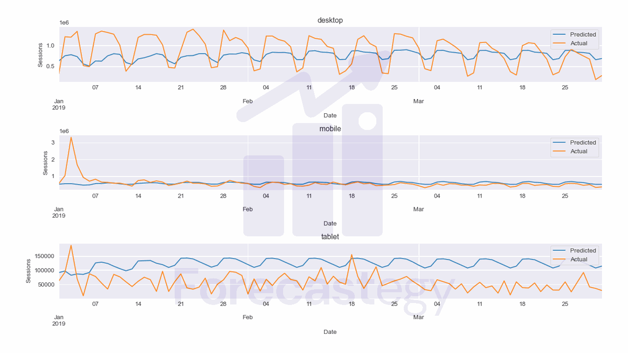
This model has a MAPE of 81.68% which is terrible for this data.
It seems the model is having a hard time capturing the seasonality of the data, although we have the date features.
This is worse than our XGBoost model. Even though they are the same class of models, the histogram approach of LightGBM seems to be very bad for this data.
Let’s see if we can improve it by tuning the hyperparameters of LightGBM.
Tuning LightGBM Hyperparameters With Optuna
Let’s use Optuna which is a straightforward hyperparameter tuning library in Python.
We need to pack our code inside an objective function that takes the trial object as an argument.
This object encapsulates one step of the optimization process.
import optuna

def objective(trial):
    learning_rate = trial.suggest_loguniform('learning_rate', 1e-3, 1e-1)
    num_leaves = trial.suggest_int('num_leaves', 2, 256)
    min_data_in_leaf = trial.suggest_int('min_data_in_leaf', 1, 100)
    bagging_fraction  = trial.suggest_uniform('bagging_fraction', 0.1, 1.0)
    colsample_bytree = trial.suggest_uniform('colsample_bytree', 0.1, 1.0)
    lags = trial.suggest_int('lags', 14, 56, step=7)

    models = [LGBMRegressor(random_state=0, n_estimators=500, bagging_freq=1,
                            learning_rate=learning_rate, num_leaves=num_leaves,
                            min_data_in_leaf=min_data_in_leaf, bagging_fraction=bagging_fraction,
                            colsample_bytree=colsample_bytree)]


    model = MLForecast(models=models,
                    freq='D',
                    lags=[1,7, lags],
                    lag_transforms={
                       1: [(rolling_mean, 7), (rolling_max, 7), (rolling_min, 7)],
                   },
                    date_features=['dayofweek', 'month'],
                    num_threads=6)


    model.fit(train, id_col='unique_id', time_col='ds', target_col='y', static_features=[])

    p = model.predict(horizon=h)
    p = p.merge(valid[['unique_id', 'ds', 'y']], on=['unique_id', 'ds'], how='left')

    error = mean_absolute_percentage_error(p['y'], p['LGBMRegressor'])

    return error
For each hyperparameter we want to tune, we use the trial.suggest_* methods.
This will sample a value for the hyperparameter from the specified distribution with different strategies that we can choose.
For now I will use the default strategy which is Tree-structured Parzen Estimator.
This is a very good sequential model-based optimization algorithm that became popular in 2011 when it was used to tune neural networks better than humans.
The ranges I picked for each hyperparameter are based on my experience with LightGBM.
I added a lags hyperparameter to show that you can tune any number that is used in your code.
I am tuning the longest lag we are using, but we could tune everything, even the window sizes of the rolling transforms or which transforms to use.
Fixing the n_estimators to 500 and tuning the learning rate tends to work better than trying to tune both at the same time.
num_leaves and min_data_in_leaf are the parameters that control the complexity of the model.
Higher num_leaves means the trees will have more nodes and will be more complex, which can lead to overfitting if done without care.
On the other hand, min_data_in_leaf controls the minimum number of samples in each leaf, which limits the number of nodes, as they have a threshold to split.
bagging_fraction and colsample_bytree are the parameters that control what randomly sampled percentage of the data is used to train each tree.
This helps reduce overfitting too.
After we define the objective function, we can create the study object and pass the objective function to it.
study = optuna.create_study(direction='minimize')
study.optimize(objective, n_trials=20)
As we return the MAPE in the objective function, we want to minimize it.
Doing about 20-30 trials is enough to get a good set of hyperparameters.
After the optimization process is done, we can get a dictionary with the best hyperparameters by using the best_params attribute.
study.best_params
{'learning_rate': 0.04982758265243196,
  'num_leaves': 172,
  'min_data_in_leaf': 31,
  'bagging_fraction': 0.9949519025635238,
  'colsample_bytree': 0.5215689568952989,
  'lags': 28},
And the best value of the objective function is in the best_value attribute.
study.best_value
0.8535369597153767
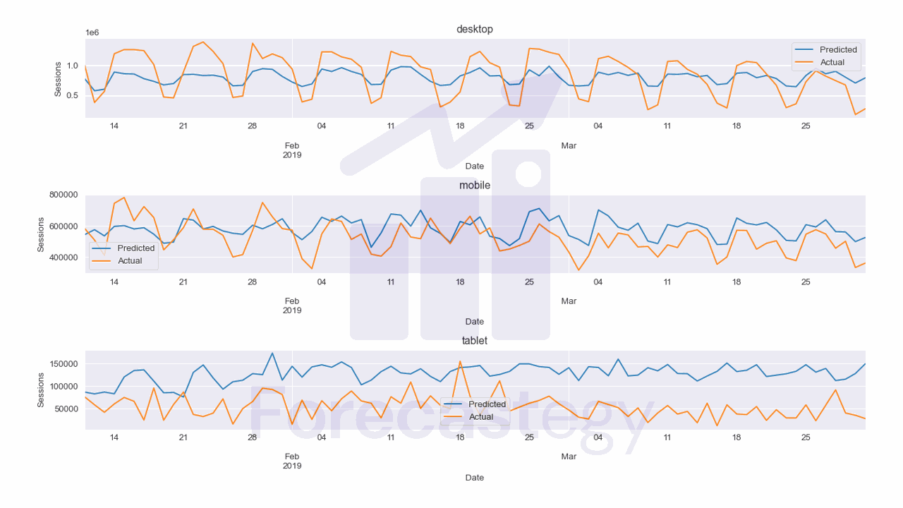
I excluded the first 10 days of data so we can see the mobile forecast better without the peak.
You can now retrain the model with the best hyperparameters and save it for later use.
As you can see the MAPE is now 85.4% which is still terrible.
For this specific dataset, a simpler model like ARIMA, Prophet or even a Seasonal Naive model might be better.
Do not use a fancy model just because you can. Use whatever works best for your data.
This is the code to plot the forecast.
fig,ax = plt.subplots(3,1,figsize=(1280/96, 720/96), dpi=96)
for ax_, device in enumerate(p['unique_id'].unique()):
    p_ = p.loc[p['unique_id'] == device]
    p_.rename(columns={'LGBMRegressor': 'Predicted', 'y': 'Actual'}, inplace=True)
    p_.plot(x='ds', y=['Predicted', 'Actual'], ax=ax[ax_], title=device)
    ax[ax_].set_xlabel('Date')
    ax[ax_].set_ylabel('Sessions')
fig.tight_layout()
Multivariate Time Series Forecasting With LightGBM in Python
You can use the same code to add more features to the model or check this tutorial on multivariate time series forecasting in Python.