Forecasting multiple time series can be a daunting task, especially when dealing with large amounts of data.
However, XGBoost is a powerful gradient boosting algorithm that has been shown to perform exceptionally well in time series forecasting tasks.
In combination with MLForecast, which is a scalable and easy-to-use time series forecasting library, we can make the process of training an XGBoost model for multiple time series forecasting a breeze.
Let’s dive into the step-by-step process of preparing our data, defining our XGBoost model, and training it using MLForecast in Python.
I will also cover some tips and tricks for optimizing the performance of our model, as well as how to evaluate its accuracy and make predictions for future time periods.
Let’s get started!
How To Install XGBoost And MLForecast
It’s easy to install XGBoost and MLForecast using pip:
pip install xgboost
pip install mlforecast
You can also install them using conda:
conda install -c conda-forge py-xgboost
conda install -c conda-forge mlforecast
How To Prepare Time Series Data For XGBoost In Python
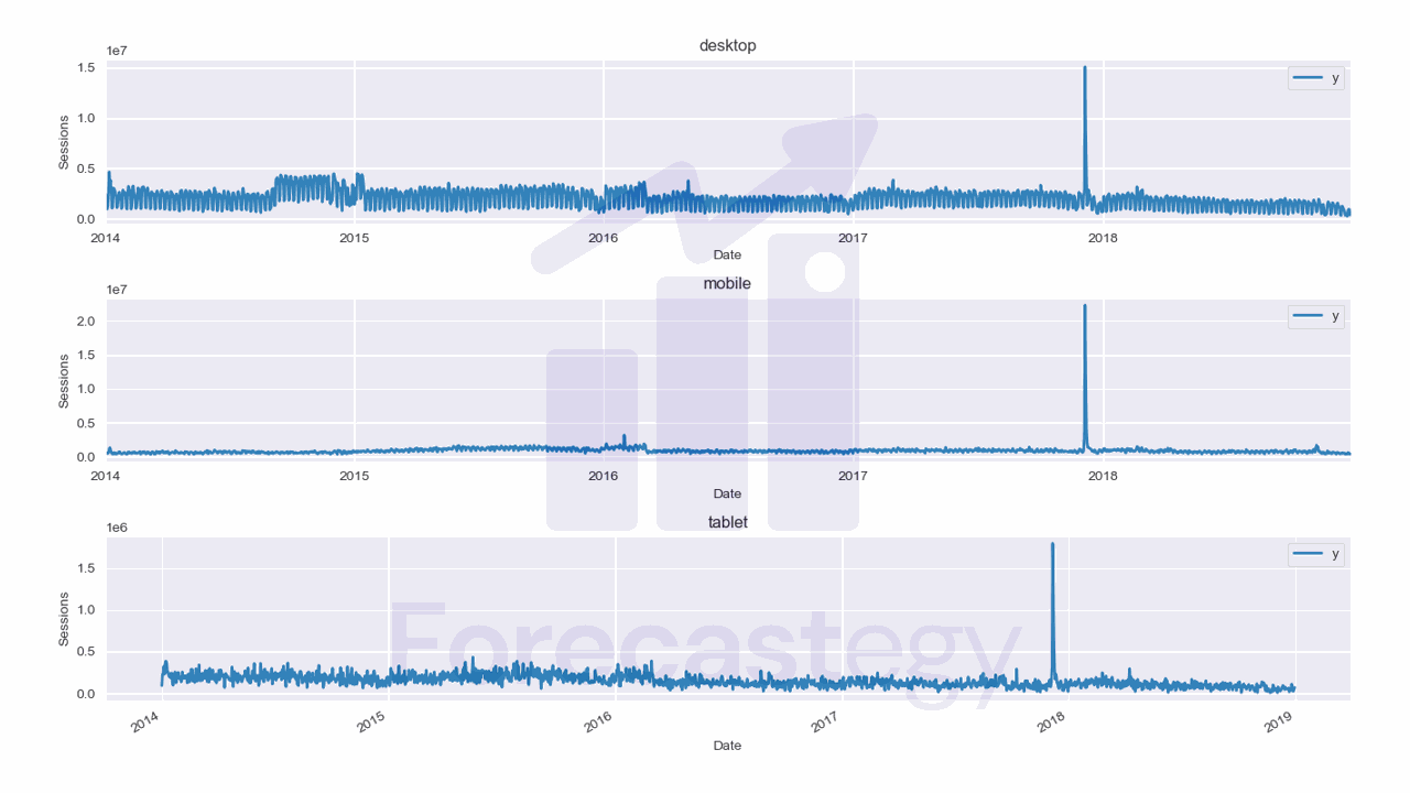
We will use data from the City of Los Angeles website traffic dataset on Kaggle.
This dataset contains the number of user sessions for the City of Los Angeles website for each day from 2014 to 2019.
Sessions are periods of time when a user is actively using the website.
Usually they are measured by looking at user activity and have a timeout after 30 minutes since the last user action.
For example, right now you are in a session on my website. If you leave the page and come back after 2 hours, you will be in a new session.
Let’s load the data and take a look at it:
import pandas as pd
import numpy as np
from matplotlib import pyplot as plt
import os

data = pd.read_csv(os.path.join(path, 'lacity.org-website-traffic.csv'),
                   parse_dates=['Date']).loc[:, ['Date', 'Device Category', 'Sessions']]
fixes = pd.DataFrame({'Date': pd.to_datetime(['2016-12-01', '2018-10-13']),
                      'Device Category': ['tablet', 'tablet'] ,
                      'Sessions': [np.nan, np.nan]})

data = pd.concat([data, fixes], axis=0, ignore_index=True)
data = data.rename(columns={'Device Category': 'unique_id', 'Sessions': 'y', 'Date': 'ds'})
data = data.sort_values(['unique_id', 'ds']).groupby('unique_id').apply(lambda x: x.fillna(method='ffill'))
| ds | unique_id | y |
|---|---|---|
| 2014-01-01 00:00:00 | desktop | 1032805 |
| 2014-01-01 00:00:00 | mobile | 537573 |
| 2014-01-01 00:00:00 | tablet | 92474 |
| 2014-01-02 00:00:00 | desktop | 2359710 |
| 2014-01-02 00:00:00 | mobile | 607544 |
We load the data with Pandas and take only 3 columns: the date, the device category, and the number of sessions.
The original data has more detailed information about the sessions, like the browser and number of visitors, but we don’t need it for this tutorial.
We then group the data by date and device category and sum the number of sessions for each group.
Here we have 3 time series: one for desktop, one for mobile, and one for tablet.
They are stacked in the long format, which means that each row represents a single observation.
This data has two points missing for the tablet device category, so we add them manually as np.nan, then fill with the previous day value.
Nixtla’s forecast libraries expect the data to have at least 3 columns: ds, unique_id, and y.
This doesn’t seem to be enforced in MLForecast, but it’s a good practice to follow.
ds is the date column, unique_id is the unique identifier for each time series, and y is the target variable.
In our case, each unique_id is a device category, but it can be an SKU, a store, a city or any other unique identifier of a time series.
Finally we split the data into train and test sets:
train = data.loc[data['ds'] < '2019-01-01']
valid = data.loc[(data['ds'] >= '2019-01-01') & (data['ds'] < '2019-04-01')]
h = valid['ds'].nunique()
I am using data from 2014 to 2018 as the training set and the first 3 months of 2019 as the validation set.
We set h to the number of days in the validation set. This is the horizon, or the number of steps we want to forecast.
This is what the training data looks like:

How To Train XGBoost For Time Series Forecasting In Python
MLForecast has a class that will handle most of the work for us.
from xgboost import XGBRegressor
from mlforecast import MLForecast

from window_ops.rolling import rolling_mean, rolling_max, rolling_min

models = [XGBRegressor(random_state=0, n_estimators=100)]

model = MLForecast(models=models,
                   freq='D',
                   lags=[1,7,14],
                   lag_transforms={
                       1: [(rolling_mean, 7), (rolling_max, 7), (rolling_min, 7)],
                   },
                   date_features=['dayofweek', 'month'],
                   num_threads=6)


model.fit(train, id_col='unique_id', time_col='ds', target_col='y', static_features=[])
We create a list with a single XGBoost model, then we create an instance of the MLForecast class.
This is the class that will handle the feature engineering and training of our model.
We can pass any of the usual hyperparameters of XGBoost to the constructor, like n_estimators and random_state, but we will use the default values for now.
We also pass the freq parameter, which is the frequency of the data. In our case, it’s daily data, so we set it to D.
The lags argument is a list of lags we want to use in our model. Lags are the number of steps in the past we want to use to predict the future.
So in our case, we are using the value of the target variable 1, 7, and 14 days before the timestamp date of the observation.
I explained the four basic features for time series forecasting in detail in the article about multiple time series forecasting with Scikit-learn.
This is why it’s important to have all dates, even the ones with missing values and zeros in the datasets, so these features can be computed correctly.
We also pass the lag_transforms argument, which is a dictionary with the lag as the key and a list of functions as the value.
These functions will be applied to the lagged series. For example, we are applying a rolling mean with a window of 7 days to the lag 1.
This means that we will have a feature that is the mean of the 7 last values of the target variable after shifting it 1 day.
You can pass any function that takes a NumPy array and returns a NumPy array. Use numba to speed up your functions, as recommended in the documentation.
I am using the window_ops library which is optimized and recommended by the developers of MLForecast.
Each tuple in the list of transforms is a function and its arguments. For example, the rolling_mean function takes a window size as its argument.
The best value for the window size is specific for each time series, so we need to try different values and see which one works best.
The date_features argument is a list of date components we want to extract from the date column.
These are important to help the model capture the seasonality of the data.
Finally, we pass the num_threads argument, which is the number of threads to use for parallel processing.
We then call the fit method to train the model.
This method takes the training data, the names of the unique identifier column, the date column, and target column, and a list of static features.
If you have no static features, pass an empty list.
To get the forecast, we call the predict method:
p = model.predict(horizon=h)
p = p.merge(valid[['unique_id', 'ds', 'y']], on=['unique_id', 'ds'], how='left')
| unique_id | ds | XGBRegressor | y |
|---|---|---|---|
| desktop | 2019-01-01 00:00:00 | 789087 | 315674 |
| desktop | 2019-01-02 00:00:00 | 1.03082e+06 | 1.20916e+06 |
| desktop | 2019-01-03 00:00:00 | 894289 | 1.19998e+06 |
| desktop | 2019-01-04 00:00:00 | 847330 | 1.33997e+06 |
| desktop | 2019-01-05 00:00:00 | 545207 | 516879 |
We pass the horizon as the argument, which is the number of steps we want to forecast.
The predict method returns a Pandas DataFrame with the predictions, so I merged it with the validation data to make it easier to evaluate the model.
from sklearn.metrics import mean_absolute_percentage_error
mean_absolute_percentage_error(p['y'], p['XGBRegressor'])
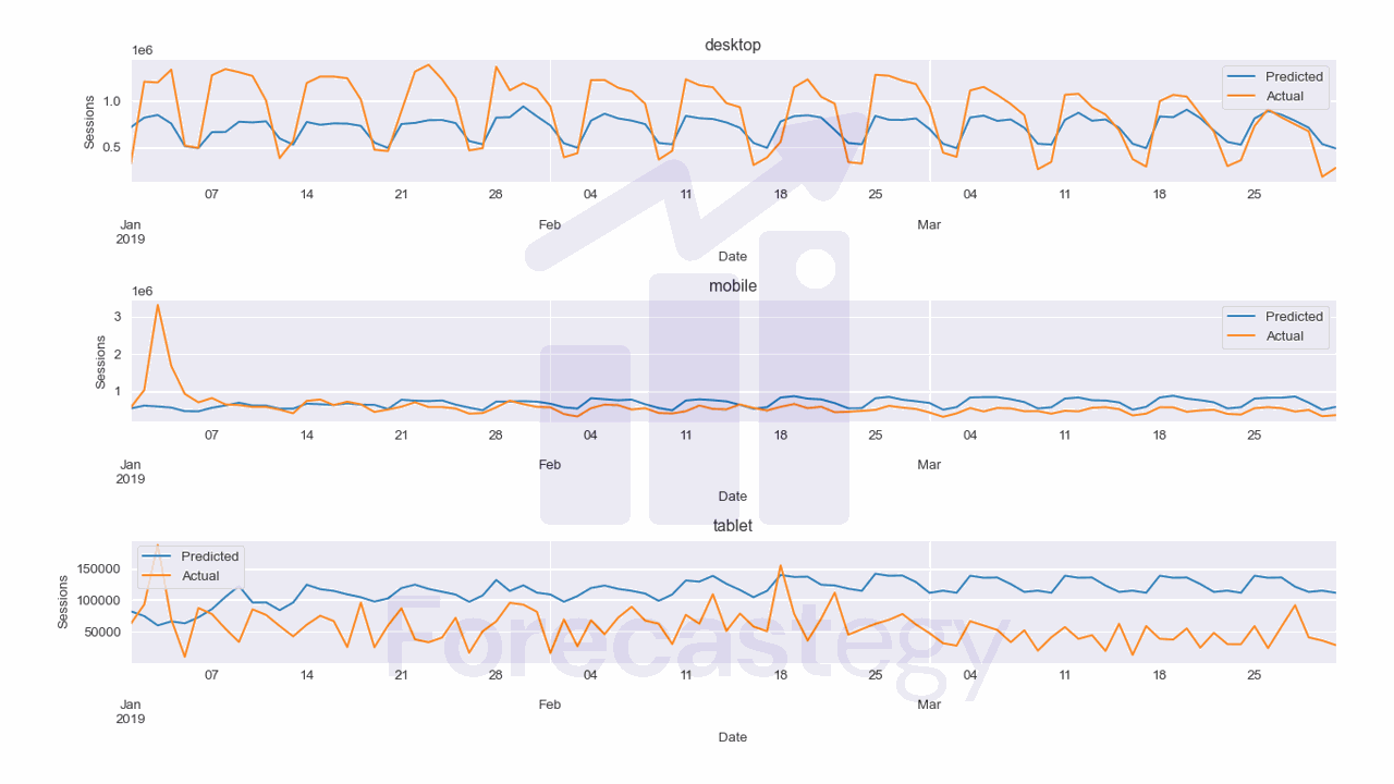
This model has a MAPE of 78.43% which is terrible for this data.
It seems the model is having a hard time capturing the seasonality of the data, although we have the date features.
Another reason for the bad performance might be the different scales of the target variable across time series.
Let’s see if we can improve it by tuning the hyperparameters of XGBoost.
How To Tune XGBoost Hyperparameters With Optuna
Let’s use Optuna which is a straightforward hyperparameter tuning library in Python.
We need to pack our code inside an objective function that takes the trial object as an argument.
This object encapsulates one step of the optimization process.
import optuna

def objective(trial):
    learning_rate = trial.suggest_loguniform('learning_rate', 1e-3, 1e-1)
    max_depth = trial.suggest_int('max_depth', 3, 10)
    min_child_weight = trial.suggest_int('min_child_weight', 1, 10)
    subsample = trial.suggest_uniform('subsample', 0.1, 1.0)
    colsample_bytree = trial.suggest_uniform('colsample_bytree', 0.1, 1.0)

    lags = trial.suggest_int('lags', 14, 56, step=7) # step means we only try multiples of 7 starting from 14

    models = [XGBRegressor(random_state=0, n_estimators=500,    learning_rate=learning_rate, max_depth=max_depth,
                           min_child_weight=min_child_weight, subsample=subsample, colsample_bytree=colsample_bytree)]

    model = MLForecast(models=models,
                    freq='D',
                    lags=[1,7, lags],
                    lag_transforms={
                       1: [(rolling_mean, 7), (rolling_max, 7), (rolling_min, 7)],
                   }, # removing this is better
                    date_features=['dayofweek', 'month'],
                    num_threads=6)


    model.fit(train, id_col='unique_id', time_col='ds', target_col='y', static_features=[])

    p = model.predict(horizon=h)
    p = p.merge(valid[['unique_id', 'ds', 'y']], on=['unique_id', 'ds'], how='left')

    error = mean_absolute_percentage_error(p['y'], p['XGBRegressor'])

    return error
For each hyperparameter we want to tune, we use the trial.suggest_* methods.
This will sample a value for the hyperparameter from the specified distribution with different strategies that we can choose.
For now I will use the default strategy which is Tree-structured Parzen Estimator.
This is a very good sequential model-based optimization algorithm that became popular in 2011 when it was used to tune neural networks better than humans.
The ranges I picked for each hyperparameter are based on my experience with XGBoost
I added a lags hyperparameter to show that you can tune any number that is used in your code.
I am tuning the longest lag we are using, but we could tune everything, even the window sizes of the rolling transforms or even which transforms to use.
I wrote a comment in the code to show that removing the lag_transforms argument improves the performance, but for clarity I will leave it in the code.
Fixing the n_estimators to 500 and tuning the learning rate tends to work better than trying to tune both at the same time.
max_depth and min_child_weight control how deep (and complex) each tree can be.
Deeper trees can capture more complex patterns, but they are more likely to overfit.
On the other hand, limiting the number of samples in each leaf node can help prevent overfitting because the tree can’t grow unless it has enough samples to split.
subsample and colsample_bytree define what percentage of the samples and features to randomly sample before building each tree.
This is a very good way to prevent overfitting.
After we define the objective function, we can create the study object and pass the objective function to it.
study = optuna.create_study(direction='minimize')
study.optimize(objective, n_trials=20)
As we return the MAPE in the objective function, we want to minimize it.
This is the output of the optimization process.
[I 2023-02-27 13:23:54,038] A new study created in memory with name: no-name-30c7e881-9eb5-429d-a843-6b2d27bf419c
[I 2023-02-27 13:23:55,569] Trial 0 finished with value: 2.336111436615988 and parameters: {'learning_rate': 0.002097538418728778, 'max_depth': 10, 'min_child_weight': 4, 'subsample': 0.34974111489122356, 'colsample_bytree': 0.3785850588954579, 'lags': 42}. Best is trial 0 with value: 2.336111436615988.
...
[I 2023-02-27 13:24:26,667] Trial 16 finished with value: 0.8503832597552246 and parameters: {'learning_rate': 0.0030152904875409095, 'max_depth': 8, 'min_child_weight': 5, 'subsample': 0.4934159533771183, 'colsample_bytree': 0.9931852650984135, 'lags': 21}. Best is trial 14 with value: 0.5840354461878713.
Doing about 20-30 trials is enough to get a good set of hyperparameters.
After the optimization process is done, we can get a dictionary with the best hyperparameters by using the best_params attribute.
study.best_params
{'learning_rate': 0.004513790331408814,
  'max_depth': 5,
  'min_child_weight': 1,
  'subsample': 0.5448631182698337,
  'colsample_bytree': 0.9909490297254225,
  'lags': 49}
And the best value of the objective function is in the best_value attribute.
study.best_value
0.5840354461878713
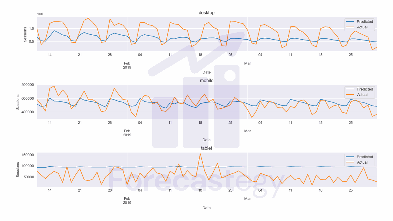
I excluded the first 10 days of data so we can see the mobile forecast better without the peak.
You can now retrain the model with the best hyperparameters and save it for later use.
As you can see the MAPE is now 58.4% which is much better than the previous model.
Still, it has difficulty capturing the seasonality of the data.
So, for this specific dataset, a simpler model like ARIMA, Prophet or even a Seasonal Naive model might be better.
Do not use a fancy model just because you can. Use whatever works best for your data.
This is the code to plot the forecast.
fig,ax = plt.subplots(3,1,figsize=(1280/96, 720/96), dpi=96)
for ax_, device in enumerate(p['unique_id'].unique()):
    p_ = p.loc[p['unique_id'] == device]
    p_.rename(columns={'XGBRegressor': 'Predicted', 'y': 'Actual'}, inplace=True)
    p_.plot(x='ds', y=['Predicted', 'Actual'], ax=ax[ax_], title=device)
    ax[ax_].set_xlabel('Date')
    ax[ax_].set_ylabel('Sessions')
fig.tight_layout()
Multivariate Time Series Forecasting With XGBoost in Python
You can use the same code to add more features to the model.
What Is The Difference Between XGBoost and Prophet For Time Series Forecasting?
XGBoost can provide powerful predictions when properly tuned and with the right feature engineering, but it requires more expertise in machine learning and data preparation.
On the other hand, Prophet is designed specifically for time series data, offers more interpretability, and requires less statistical expertise, making it easier for analysts to incorporate their domain knowledge in the forecasting process.
| Feature | XGBoost | Prophet |
|---|---|---|
| Model Type | Global (Can handle multiple time series) | Local (Handles one time series at a time) |
| Training | More complex setup (requires feature engineering and data prepping) | Easier setup (handles trend, seasonality, and holidays automatically) |
| Flexibility | Can handle various types of data/features | Designed specifically for time series data with trends, seasonality, and holidays |
| Hyperparameter Tuning | Requires tuning to achieve better performance | Offers intuitive parameters with less need for tuning |
| Performance | Can perform well with proper tuning and feature engineering | Performs well on common business time series without much tuning |
| Scalability | Can be parallelized for faster training | Has to fit one model for each time series, which can be slow |
| Interpretability | Less interpretable (due to complex features) | More interpretable (parameters related to trends, seasonality, holidays) |
| Expertise Needed | Requires more expertise in machine learning and feature engineering | Requires less statistical expertise, allows for analyst-in-the-loop modeling |
| Library | XGBoost, MLForecast | Prophet |
Model Type
XGBoost is a global model that can handle multiple time series simultaneously.
This is beneficial when you are dealing with several related time series, as it can leverage the relationships between them to improve forecasting accuracy.
On the other hand, Prophet is a local model designed to handle one time series at a time.
This means that, when working with multiple time series, you would need to fit a separate model for each series.
Training
Training an XGBoost model for time series forecasting requires a more complex setup, involving feature engineering and data prepping.
This can be time-consuming and require a deeper understanding of the data and the model’s inner workings.
In contrast, Prophet offers an easier setup, as it automatically handles trend, seasonality, and holidays within the algorithm, simplifying the process for users.
Flexibility
XGBoost is a versatile model that can handle various types of data and features.
This flexibility can be advantageous when working with diverse or non-standard datasets, as the model can be adapted to suit your needs.
Prophet, on the other hand, is designed specifically for time series data with trends, seasonality, and holidays.
While this makes it more suited for common business time series, its application may be limited in cases where the data deviates from these assumptions.
Hyperparameter Tuning
XGBoost typically requires hyperparameter tuning to achieve optimal performance.
This can be time-consuming and might demand a deeper understanding of the model and its parameters.
On the other hand, Prophet offers intuitive parameters that require less tuning, making it more accessible for analysts without extensive expertise in machine learning.
Performance
With proper tuning and feature engineering, XGBoost can deliver strong performance on time series forecasting tasks.
However, this comes with the caveat that it requires more effort and expertise to achieve these results.
Prophet, in contrast, performs well on common business time series without the need for extensive tuning, making it a more convenient option for many users.
Scalability
XGBoost can be parallelized for faster training, allowing it to handle larger datasets and more complex models more efficiently.
Prophet needs to fit one model for each time series, which can be slow and computationally expensive, making it less scalable.
Interpretability
XGBoost models, due to their complex features, can be less interpretable, making it harder for users to understand the underlying relationships in the data.
Prophet provides greater interpretability, with parameters related to trends, seasonality, and holidays, allowing analysts to better understand the model and its predictions.
Expertise Needed
XGBoost requires a higher level of expertise in machine learning and feature engineering to achieve optimal results.
This can be a barrier for some users who may not have the necessary background.
In contrast, Prophet requires less statistical expertise and allows for analyst-in-the-loop modeling, enabling forecasters to apply their domain knowledge and insights to improve the model without needing advanced skills in machine learning or statistics.
XGBoost and Prophet cater to different needs and levels of expertise.
XGBoost offers more flexibility and performance potential but requires more effort and knowledge, while Prophet is easier to use, more interpretable, and tailored