
Want to use LightGBM for a binary classification task but feel stuck?
In this tutorial, you are going to see an example of how to do it in Python step-by-step.
I’ll also explain how to handle class imbalance, a common issue in binary classification tasks.
What Is LightGBM?
LightGBM, which stands for “Light Gradient Boosting Machine,” is an open-source, distributed, high-performance gradient boosting framework developed by Microsoft.
It is designed for efficient and scalable training of large datasets and is particularly well-suited for problems involving large numbers of features or high-dimensional data.
Gradient boosting is an ensemble machine learning algorithm that builds a predictive model in the form of a set of weak learners, typically decision trees (GBDT).
LightGBM, like other gradient boosting frameworks (e.g., XGBoost), builds trees sequentially, with each tree trying to correct the errors of the previous ones.
This is different from Random Forests, which builds trees independently by randomly sampling the data with replacement and features without replacement.
Installing LightGBM in Python
Before we dive into the main content of this tutorial, let’s first ensure that you have the LightGBM library installed in your Python environment.
You can install LightGBM either using conda or pip.
If you’re using an Anaconda distribution, you can install LightGBM by using the following command in your terminal:
conda install -c conda-forge lightgbm
If you prefer using pip, run this command:
pip install lightgbm
After running one of these commands, LightGBM should be installed and ready for use in your Python environment.
Preparing the Data
The first step in any machine learning project is to load the data.
We’ll be using the Adult Dataset for this tutorial.
You can load this dataset into a pandas DataFrame using the read_csv function.
Here’s how you can do it:
import pandas as pd

data = pd.read_csv('adult.csv')
Splitting the Data into Training and Testing Sets
Once you’ve loaded the data, the next step is to split it into a training set and a testing set.
This allows us to evaluate the performance of our model on unseen data.
We’ll use the train_test_split function from the sklearn.model_selection module to do this.
Here’s how:
from sklearn.model_selection import train_test_split

X = data.drop('income', axis=1)
y = data['income']

X_train, X_test, y_train, y_test = train_test_split(X, y, test_size=0.2, random_state=42)
In this code, we first separate the features (X) from the target variable (y).
We then split both into training and testing sets, with 80% of the data going to the training set and 20% going to the test set.
Preprocessing the Data
After splitting the data, the next step is to preprocess it.
This involves transforming categorical variables into integers and handling missing values.
To transform categorical variables into integers, we’ll use the OrdinalEncoder from the category_encoders package.
I prefer using it instead of the LabelEncoder from sklearn.preprocessing because it’s a more robust and complete implementation.
Here’s how:
import category_encoders as ce

encoder = ce.OrdinalEncoder(cols=['workclass', 'education', 'marital.status', 'occupation', 'relationship', 'race', 'sex', 'native.country'])

X_train = encoder.fit_transform(X_train)
X_test = encoder.transform(X_test)
In the above code, we first initialize the OrdinalEncoder specifying the columns we want to transform.
We then fit this encoder to the training data and transform it. We also transform the test data using the same encoder.
It will not only transform the categorical variables into integers but also concatenate the transformed columns to the other (numerical) columns.
If you don’t have the category_encoders package installed, you can install it by running the following command in your terminal:
pip install category_encoders
or
conda install -c conda-forge category_encoders
To handle missing values, we’ll replace them with NaNs.
import numpy as np

X_train = X_train.replace('?', np.nan)
X_test = X_test.replace('?', np.nan)
In this code, we replace any ‘?’ in the data with ‘NaN’ using the replace function.
This is because LightGBM can handle missing values represented as np.nan by default.
Building the Model
When building a LightGBM model, there are several hyperparameters that you can tune.
However, for the purpose of this tutorial, we will focus on three of the most important ones:
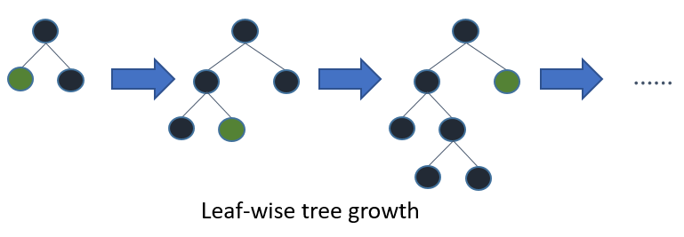
learning_rate: This is the learning rate or shrinkage rate. It controls how much each tree contributes to the overall prediction. Generally, a lower learning rate is better, but it also means that the model will take longer to train.n_estimators: This is the number of boosting rounds or trees to build. It controls the complexity of the model. I like to set as high a value as possible for this parameter, but it also means that the model will take longer to train.num_leaves: This is the main parameter to control the complexity of the tree model. It controls the number of leaves in each tree, which is a proxy for the depth. A higher value means a more complex, less regularized model, which can lead to overfitting.
To set the hyperparameters, we create an LGBMClassifier object and pass in the hyperparameters as arguments.
from lightgbm import LGBMClassifier

lgb = LGBMClassifier(learning_rate=0.05, n_estimators=100, num_leaves=31)
Binary vs Cross-Entropy Objective
LightGBM offers two loss functions for binary classification: binary and cross_entropy.
Most of the time you will use binary, which optimizes the log loss when your classes are labeled with only 0s and 1s.
If you want to optimize probabilities directly (as labels), you can use cross_entropy.
This loss function will consider multiple labels with values between 0 and 1 as probabilities of the positive class.
It’s rare, but one use case is when you have probabilities from another model and want to train a LightGBM model to match those probabilities instead of the binary labels.
Using is_unbalance To Handle Class Imbalance
If your dataset is imbalanced (has many more instances of one class than the other), you can use the is_unbalance parameter to handle it.
Setting it to True will multiply the weight of the positive class errors by the ratio of negative to positive instances in the dataset, making the model pay more attention to the under-represented class.
To use this parameter, you simply set it to True when initializing the LGBMClassifier object.
lgb = LGBMClassifier(learning_rate=0.05, n_estimators=100, num_leaves=31, is_unbalance=True)
Be warned that, although it improves metrics like ROC AUC, it will hurt metrics like log loss, due to it breaking the probability calibration of the predictions.
So, a rule of thumb is, if you only care about positive samples having a higher predicted score than negative samples, then you can use is_unbalance=True.
If you want your predictions to be closer to the real probabilities of the classes, then you should set is_unbalance=False.
Training the Model
Once you’ve set your hyperparameters, you can train your LightGBM model using the fit method.
LightGBM can handle raw integer-encoded categorical features well by default.
However, you can set the categorical_feature parameter to the column names of the categorical features.
In practice, try both ways and see which one performs better.
Here’s how to do it:
lgb.fit(X_train, y_train, categorical_feature=['workclass', 'education', 'marital.status', 'occupation', 'relationship', 'race', 'sex', 'native.country'])
In this code, we just pass the training data and the list of categorical features to the fit method.
Some people like to do early stopping when training LightGBM models, but in my experience, it tends to overfit badly with gradient boosting models.
Making Predictions
Class Predictions
Once the model is trained, you can use it to make predictions.
If you want to directly predict the class for each instance in the test set, you can use the predict function of the model.
y_pred = lgb.predict(X_test)
The predict function applies a threshold of 0.5 to the predicted probabilities.
So each instance will be assigned a class of 1 if the predicted probability of the positive class is greater than 0.5, and a class of 0 otherwise.
Probability Predictions
If you’re interested in the predicted probabilities rather than the class predictions, you can use the predict_proba function of the model.
probabilities = lgb.predict_proba(X_test)[:, 1]
By default, this function returns an array with two columns, one for the probability of the negative class and one for the probability of the positive class.
This is why we take the second column using the [:, 1] syntax.
Evaluating the Model
After making predictions with your model, the next step is to evaluate its performance.
There are several metrics you can use for this, including accuracy, log loss, ROC AUC, and the classification report.
Accuracy
Accuracy is the most straightforward metric.
It’s simply the proportion of predictions that the model got right.
from sklearn.metrics import accuracy_score

accuracy = accuracy_score(y_test, y_pred)
print('Accuracy: ', accuracy)
However, there are many other metrics that are more informative than accuracy, especially when dealing with imbalanced datasets.
Log Loss
Log loss, also known as logistic loss or cross-entropy loss, is a performance metric for evaluating the predicted probabilities of membership to a given class.
from sklearn.metrics import log_loss

loss = log_loss(y_test, probabilities)
print('Log loss: ', loss)
ROC AUC
The ROC AUC score provides an aggregate measure of performance across all possible classification thresholds.
from sklearn.metrics import roc_auc_score

roc_auc = roc_auc_score(y_test, probabilities)
print('ROC AUC: ', roc_auc)
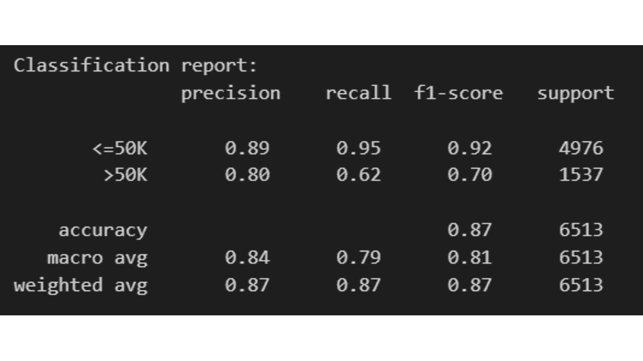
Classification Report
The classification report displays the precision, recall, F1, and support scores for the model.
from sklearn.metrics import classification_report

report = classification_report(y_test, y_pred)
print('Classification report: \n', report)
If you want more fine-grained information of which classes are being predicted correctly and which ones are not, you can use a confusion matrix.
Confusion Matrix
A confusion matrix is a table that summarizes the performance of a classification model on a set of test data for which the true values are known.
from sklearn.metrics import confusion_matrix

matrix = confusion_matrix(y_test, y_pred)
print('Confusion matrix: \n', matrix)
By evaluating your model using these metrics, you can get a good understanding of its performance across different aspects.
It’s worth noting that LightGBM can be used for regression and multi-class classification as well.