In this post, we will learn how to use DeepAR to forecast multiple time series using GluonTS in Python.
DeepAR is a deep learning algorithm based on recurrent neural networks designed specifically for time series forecasting.
It works by learning a model based on all the time series data, instead of creating a separate model for each one.
In my experience, this often works better than creating a separate model for each time series.
The model is based on an autoregressive architecture, which means that it uses information from previous time steps to predict future values.
It has two parts: an encoder network, which remembers what it has seen, and a decoder network, which predicts what will happen next.
It learns a conditional distribution over the future values and uses a recursive approach to generate predictions for multiple time steps.
So instead of simply predicting a point estimate, it samples values from the learned distribution and uses that as the prediction.
Installing GluonTS
I recommend you first install PyTorch or MXNet, as GluonTS is built on top of these frameworks.
In this tutorial I will use the PyTorch backend as it’s more popular and easy to install on Windows, Mac and Linux.
Check these instructions to install PyTorch.
Then we need to install PyTorch Lightning, which is a lightweight PyTorch wrapper for high-performance AI research.
You can use pip:
pip install pytorch-lightning
Or conda:
conda install pytorch-lightning -c conda-forge
Finally, we can install GluonTS:
pip install gluonts
Now we are ready to start!
Preparing Multiple Time Series Data For DeepAR
We will use real sales data from the Favorita store chain, from Ecuador.
We have sales data from 2013 to 2017 for multiple stores and product categories.
To measure the model’s performance, we will use WMAPE (Weighted Mean Absolute Percentage Error) with the absolutes of the actual values as weights.
import pandas as pd
import numpy as np

def wmape(y_true, y_pred):
    return np.abs(y_true - y_pred).sum() / np.abs(y_true).sum()
This is an adapted version of MAPE (Mean Absolute Percentage Error) that solves the problem of division by zero when there are no sales for a specific day.
For this tutorial I will use only the data from one store.
You can use as many stores, categories, SKUs, etc as you want.
data = pd.read_csv(os.path.join(path, 'train.csv'), index_col='id', parse_dates=['date'])
data2 = data.loc[data['store_nbr'] == 1, ['date', 'family', 'sales']]
The columns are:
date: date of the recordfamily: product categorysales: sales amount
This data doesn’t contain a record for December 25, so I added a record for each year and product category.
dec25 = list()
for year in range(2013,2017):
    for family in data2['family'].unique():
        dec25 += [{'date': pd.Timestamp(f'{year}-12-25'), 'family': family, 'sales': np.nan}]
data2 = pd.concat([data2, pd.DataFrame(dec25)], ignore_index=True).sort_values('date')
This is how the data looks like:
| date | family | sales |
|---|---|---|
| 2013-01-01 00:00:00 | AUTOMOTIVE | 0 |
| 2013-01-01 00:00:00 | SEAFOOD | 0 |
| 2013-01-01 00:00:00 | SCHOOL AND OFFICE SUPPLIES | 0 |
| 2013-01-01 00:00:00 | PRODUCE | 0 |
| 2013-01-01 00:00:00 | PREPARED FOODS | 0 |
One row per day per product category.
GluonTS requires a minimum of two columns: the timestamp and the target.
We do a simple time series split into train and validation sets.
train = data2.loc[data2['ds'] < '2017-01-01']
valid = data2.loc[(data2['ds'] >= '2017-01-01') & (data2['ds'] < '2017-04-01')]
To use the data as input for DeepAR, we need create a dataset with the PandasDataset class.
from gluonts.dataset.pandas import PandasDataset

train_ds = PandasDataset.from_long_dataframe(train, target='sales', item_id='family',
                                       timestamp='date', freq='D')
This will take a Pandas dataframe in the long format, which means that each row is a single observation in time like you saw above.
The first argument is the dataframe.
Then we pass the name of the column with the time series values as target.
The item_id is the name of the column with the time series identifier.
In our case we have one time series per product category, but this could be SKUs, stores, a mix of all of them, etc.
The timestamp is the name of the column with the timestamp.
Finally, we pass the freq argument, which is the frequency of the time series.
DeepAR’s Important Hyperparameters
Before we train a DeepAR model, it’s important to understand which levers we can pull to improve the model’s performance and their default values.
These are hyperparameters you can tune manually or with my favorite methods: Bayesian Optimization and Random Search.
num_layers
This is the number of layers in the RNN.
Just like a feedforward neural network, a recurrent neural network can have multiple layers to learn more complex patterns as it goes deeper.
More layers means more capacity to learn, but also more time to train and a higher risk of overfitting.
The default value is 2.
hidden_size
This is the number of units (neurons) in each layer of the RNN.
Again, you can think about it just like the hidden layers in a feedforward neural network.
So if you have 2 layers of 10 units each, you have a total of 20 units.
The default value is 40, which means 40 units in each layer, not in total.
context_length
This is the number of time steps the model will use as inputs to predict the next time step.
For example, if you have a daily time series and you set context_length=30, the model will use the last 30 days to predict the next day.
The default value is None which means the model will use the same size as the prediction horizon (how many steps ahead you want to predict).
prediction_length
This is the number of time steps you want to predict, the same as the prediction horizon.
This is usually not something you tune, but you decide based on the problem you are trying to solve.
If you need to manage the inventory of a store for the next 30 days, you would set prediction_length=30.
There is no default value for this.
lr
This is the learning rate of the optimizer.
An extremely important hyperparameter in any deep learning model, the learning rate controls how much the model learns at each step.
A low learning rate will make the model learn slowly, but it will also make it more stable.
A high learning rate will make the model learn faster, but it can make it jump around the minimum and never converge.
The default value is 0.001.
weight_decay
This is the regularization parameter for the weights during training.
A higher value means more regularization, which will help prevent overfitting, but if you set it too high, the model will be too limited to learn anything.
The default value is 1e-8.
dropout_rate
This is another regularization parameter.
Dropout is a very successful regularization technique in deep learning that randomly sets a percentage of the units in a layer to zero during training.
The percentage is controlled by the dropout_rate parameter, which by default is 0.1.
Again, higher values mean more regularization, but if you set it too high, the model will have a hard time learning anything.
Training DeepAR With Multiple Time Series in GluonTS
Now that we prepared the data and checked the hyperparameters, we can train a DeepAR model.
from gluonts.torch.model.deepar import DeepAREstimator

estimator = DeepAREstimator(freq='D', prediction_length=90, num_layers=3, trainer_kwargs={'accelerator': 'gpu', 'max_epochs':30})

predictor = estimator.train(train_ds, num_workers=2)
The first thing we do is create an instance of the DeepAREstimator class.
We pass the frequency of the time series, the prediction horizon, and any hyperparameter we want to change from the default values.
I set num_layers=3 to show you how to pass a custom value for a hyperparameter. You can do it with any of the ones we discussed above.
Then we pass the trainer_kwargs argument, which is a dictionary with the arguments we want to pass to the Trainer class from PyTorch Lightning.
In this case, I set accelerator='gpu' to use a GPU for training, and max_epochs=30 to limit the number of epochs to 30.
I am not a big fan of early stopping, so I prefer to set a fixed number of epochs, change other parameters and see how the model performs on the validation set.
Then we call the train method to train the model.
Notice that, different from the usual scikit-learn API, the train returns a predictor object, which contains the trained model we need to make predictions.
You can pass the argument num_workers to use multiple CPU cores to process the data in parallel.
Generating Forecasts With DeepAR in GluonTS
Now that we have a trained model, we can use it to make predictions.
pred = list(predictor.predict(train_ds))
The predict method from the predictor object takes a dataset as input and returns a generator with the predictions.
So I just converted it to a list to make it easier to work with.
This list has one element (SampleForecast) for each time series in the dataset.
gluonts.model.forecast.SampleForecast(info=None, item_id='AUTOMOTIVE', samples=array([[ 2.62961888e+00,  5.79311228e+00,  4.37896729e+00, ...,
         1.35754282e-02,  7.44775077e-03,  9.93073732e-03],
       [ 6.60183430e+00,  6.32119608e+00,  8.18489933e+00, ...,
         1.81828451e+00,  5.14256239e+00, -6.12959921e-01],
       [ 2.50267696e+00,  3.27369547e+00,  5.98513556e+00, ...,
         4.69780779e+00,  1.05829077e+01,  2.56207967e+00],
       ...,
       [ 2.67228460e+00, -1.20100975e+01,  1.10680330e+00, ...,
         3.05511360e-03,  9.52694472e-03,  1.56723391e-02],
       [ 8.64363253e-01,  5.00162697e+00,  3.46997476e+00, ...,
         3.64174962e+00,  5.12161493e+00,  3.03343010e+00],
       [-3.41650271e+00, -2.11985683e+00,  1.45359602e+01, ...,
         9.26697075e-01,  3.74575925e+00, -2.79996371e+00]], dtype=float32), start_date=Period('2017-01-01', 'D'))
This object contains the predictions for the time series, the start date of the prediction, and the item id.
We will use it all to build a dataframe with the predictions later.
Notice that I am passing the training dataset as input.
In many other libraries this would predict the examples in the training set, but in this case it will use the last context_length time steps from it to predict the prediction_length time steps ahead in a recursive fashion.
If you never heard of recursive or autoregressive predictions in time series forecasting with machine learning, it just means that the model will predict one step ahead, then use the prediction as input to predict the next step, and so on.
So the predictions become observations in the input sequence for the next prediction until we reach the prediction_length.
all_preds = list()
for item in pred:
    family = item.item_id
    p = item.samples.mean(axis=0)
    p10 = np.percentile(item.samples, 10, axis=0)
    p90 = np.percentile(item.samples, 90, axis=0)
    dates = pd.date_range(start=item.start_date.to_timestamp(), periods=len(p), freq='D')
    family_pred = pd.DataFrame({'date': dates, 'family': family, 'pred': p, 'p10': p10, 'p90': p90})
    all_preds += [family_pred]
all_preds = pd.concat(all_preds, ignore_index=True)
all_preds = all_preds.merge(valid, on=['date', 'family'], how='left')

wmape(all_preds['sales'], all_preds['pred'])
We iterate over the pred list to build a dataframe with the predictions.
From each SampleForecast object we extract the item id, the predictions, and the dates.
Because DeepAR returns 100 samples for each time step, we need to take the mean of the predictions to get the most likely value.
The cool thing is that we can also create uncertainty intervals for the predictions.
Here I am using the 10th and 90th percentiles of the samples.
Finally, we merge the predictions with the validation set to compare them with the actual values and make it easier to plot the results.
This is what all_preds look like at the end:
| date | family | pred | p10 | p90 | sales |
|---|---|---|---|---|---|
| 2017-01-01 00:00:00 | AUTOMOTIVE | 2.24534 | -1.49905 | 5.09982 | 0 |
| 2017-01-02 00:00:00 | AUTOMOTIVE | 3.34988 | -0.124339 | 7.70383 | 5 |
| 2017-01-03 00:00:00 | AUTOMOTIVE | 4.81404 | -0.177619 | 9.76908 | 4 |
| 2017-01-04 00:00:00 | AUTOMOTIVE | 4.7317 | 2.01581 | 7.55012 | 1 |
| 2017-01-05 00:00:00 | AUTOMOTIVE | 4.01265 | 1.04238 | 8.33445 | 2 |

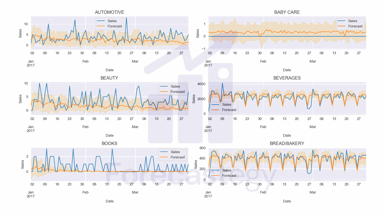
I used the following code to plot the results for a few families with their uncertainty intervals:
fig, ax = plt.subplots(3,2, figsize=(1280/96, 720/96), dpi=96)
ax = ax.flatten()
for ax_ ,family in enumerate(all_preds['family'].unique()[:6]):
    p_ = all_preds.loc[all_preds['family'] == family]
    p_.plot(x='date', y='sales', ax=ax[ax_], label='Sales')
    p_.plot(x='date', y='pred', ax=ax[ax_], label='Forecast')
    ax[ax_].fill_between(p_['date'].values, p_['p10'], p_['p90'], alpha=0.2, color='orange')
    ax[ax_].set_title(family)
    ax[ax_].legend()
    ax[ax_].set_xlabel('Date')
    ax[ax_].set_ylabel('Sales')
fig.tight_layout()
DeepAR seems to capture the seasonality pretty well in this data, but struggles a bit with items that have a low number of sales.
Tuning the hyperparameters of the model or creating separate models for low and high sales items could help.
What Is The Difference Between DeepAR and Prophet?
DeepAR is a global model, meaning that it learns a single model for all time series in your dataset.
It leverages information from all available time series to make predictions for each individual time series.
This can be beneficial, especially when you have multiple related time series and would like to leverage the patterns found in one series to help predict another.
Prophet, on the other hand, is a local model.
It fits an individual model for each time series in your dataset.
Although this approach may require more computational resources, it allows for greater flexibility in modeling unique characteristics of each individual time series.
As for handling additional covariates, both DeepAR and Prophet can incorporate external information through covariates.
Here’s a table comparing DeepAR and Prophet based on ten relevant aspects:
| Aspect | DeepAR | Prophet |
|---|---|---|
| Model Type | Global (Single model for all time series) | Local (Individual model for each time series) |
| Covariates | Item-dependent, time-dependent, or both | Additional regressors can be added |
| Data Type and Scale | Handles a wide range of scales and types | Designed for common business time series data |
| Ease of Use | Requires some knowledge of recurrent networks | Intuitive parameters, easier for non-experts |
| Domain Knowledge | Not explicitly designed for expert input | Analyst-in-the-loop approach for expert input |
| Seasonality Detection | Learns seasonality patterns automatically | Handles multiple seasonalities using Fourier series |
| Handling Holidays | Not built-in, but can be included as covariates | Built-in holiday effects with custom lists |
| Computational Efficiency | Suitable for large-scale datasets | Can be slower for a large number of time series |
| Uncertainty Estimation | Provides uncertainty estimates | Provides uncertainty intervals |
| Open-Source Availability | Open-source available and SageMaker Proprietary version | Open-source software in Python and R |
This table offers additional aspects to consider when comparing DeepAR and Prophet.
As before, the best choice will depend on your specific forecasting needs and the characteristics of your data.
Trying both models on a sample of your data and comparing their performance can help you determine which one is the most suitable for your purposes.