Some posts ago, I shared about a competition sponsored by Criteo that I decided to participate in to learn more about the out-of-distribution robustness of machine learning models.
It turns out I got 3rd place and a prize!
In any competition, you need to write a report on your solution to claim the prize, so I decided to post it here too.
Enjoy!
Background
The competition had a dataset with about 40 categorical features “aggregated from traces in computational advertising” and a binary target. We could be predicting clicks on ads, for example.
It is an out-of-distribution generalization challenge for ECML-PKDD 22, so the final results were computed over a test set that didn’t come from the same distribution as the training set.
When you see LB or Dev Never-Seen Environment, it’s about the dataset with a different distribution in which we could see the score during the competition.
When you see LB Train Envs, it’s about the score in an out-of-sample data that came from the same distribution as the training set.
When you see LB Final or simply Final, it’s about the dataset with a different distribution that was revealed after the competition finished (and was used to define the winners).
LB means leaderboard. Two during the competition and one after.
We had data from 3 different distributions (environments) in the training set.
Preprocessing
The binary features were kept in their original format.
For the boosted tree models, categorical features with more than 2 values were transformed using Ordinal Encoding and Count Encoding.
Ordinal encoding (OE) sorts the values alphabetically and simply replaces the original categorical value with a number sequentially according to the sorting.
Count encoding (CE) computes the number of rows for each categorical value and replaces the original categorical value with this number.
For the benchmark logistic regression, the organizers used the hashing trick to transform the categorical values into numerical ones.
It assigns them to buckets with a hash function, then uses this transformed representation to train models. They used scikit-learn’s FeatureHasher with 2**15 buckets and the option alternate_sign set to False.
After the hashing, the resulting columns were scaled by dividing their values by the maximum absolute value of the respective column with the MaxAbsScaler object from scikit-learn.
Validation
Following the findings of Gulrajani and David’s paper I shared on the previous post, the original training set was randomly split into 5 folds for cross-validation.
All models were evaluated using this method.
XGBoost
XGBoost was trained with default parameters but 1,000 estimators and max_bin = 1024.
Max_bin defines how many buckets will be used to preprocess the features to speed up training but can be thought of as a regularization mechanism. The training was done using a GPU on Google Colab.
The features were a concatenation of OE and CE. Optimization loss was cross-entropy.
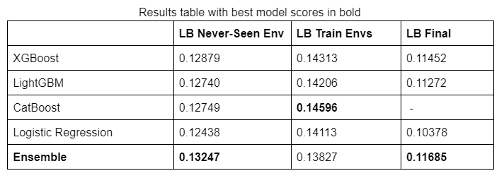
This model had a Normalized Cross-Entropy of 0.14977 averaged over the 5 folds, 0.12879 on the Dev Never-Seen Environment, and 0.11452 as the Final score.
LightGBM
LightGBM was trained with default parameters but 1,000 estimators. The idea with LightGBM and CatBoost was to get different predictions for the ensemble.
The features were a concatenation of OE and CE. Optimization loss was cross-entropy.
This model had a Normalized Cross-Entropy of 0.15116 averaged over the 5 folds, 0.12740 on the Dev Never-Seen Environment, and 0.11272 as the Final score.
CatBoost
CatBoost was trained with default parameters but 2,000 estimators.
The features were OE with the attribute cat_cols set to all columns. This allows Catboost to use its internal target encoding to transform the features. Optimization loss was cross-entropy.
This model had a Normalized Cross-Entropy of 0.15348 averaged over the 5 folds, 0.12749 on the Dev Never-Seen Environment. Final score was not reported.
Logistic Regression
This model was trained for a maximum of 1,000 iterations.
The inverse regularization coefficient was set to 1 over the average of the Euclidean norms of the first 10,000 rows of the training set.
The raw features were preprocessed with the hashing trick and scaled, as noted in the preprocessing section.
This model had a Normalized Cross-Entropy of 0.14795 averaged over the 5 folds, 0.12438 on the Dev Never-Seen Environment, and 0.10378 as the Final score.
Results Table With Best Model Scores In Bold
Final Ensemble
The first component of the ensemble was an average of the probabilities predicted by XGBoost, LightGBM and Catboost.
Then the logistic regression prediction was multiplied by 0.05 and subtracted from the average above.
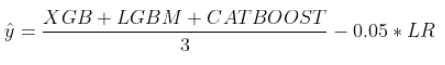
This was done to simulate “Feature Neutralization”.
The technique is well-known to the Numerai community. The basic idea is to fit a linear predictor on a subset of features and subtract its predictions from a more complex model. It reduces the influence of the fitted features and helps the model be more robust to distributions that are different from training.
A coefficient of 0.05 was found by probing the leaderboard.
It scored 0.13247 in the Dev Never-Seen Environment and 0.11685 in the Final Leaderboard, taking 3rd place.
Check the post about out-of-distribution models to see other ideas I tried and my learnings for projects outside of competitions.