
Multi-output regression is a machine learning task where we need to predict multiple outputs from a single set of inputs.
Imagine you’re a financial analyst at an investment firm.
Your job is to predict the future performance of various stocks to guide investment decisions.
For each stock, you want to predict several outputs such as the expected return, the volatility (risk), and the correlation with other stocks or market indices.
These outputs are all interrelated and depend on a common set of inputs such as the company’s financial health, market conditions, economic indicators, and so on.
In this case, you could use a multi-output regression model.
The model would take in all the relevant financial data and output the expected return, volatility, and correlation for each stock.
In this tutorial, we’re going to explore how to use XGBoost, a powerful machine learning library, to tackle this modeling problem.
I’ll walk you through the process step by step, from installing XGBoost and loading your data, to training your model and evaluating its performance.
By the end of this tutorial, you’ll have a clear understanding of how to handle multi-output regression with XGBoost.
So, let’s dive in and start learning together!
Installing XGBoost In Python
Before we can start using XGBoost, we need to install it.
XGBoost can be installed using pip, which is a package manager for Python.
To install it, you can use the following command in your terminal:
pip install xgboost
If you are using a Jupyter Notebook, you can run this command in a code cell by prefixing it with an exclamation mark:
!pip install xgboost
You can do it using conda and mamba too:
conda install -c conda-forge xgboost
mamba install -c conda-forge xgboost
After running this command, XGBoost should be installed and ready to use.
You can check if it’s installed correctly by importing it in your Python script:
import xgboost as xgb
If this command runs without any errors, congratulations! You have successfully installed XGBoost.
Loading The Data
Let’s import the necessary packages and load our dataset.
Specifically, we’re using pandas to load the data into a DataFrame and NumPy to work with arrays.
import pandas as pd
import numpy as np

data_path = "path_to_your_data"
data = pd.read_csv(data_path)
| u_q | coolant | stator_winding | u_d | stator_tooth | motor_speed | i_d | i_q | pm | stator_yoke | ambient | torque | profile_id |
|---|---|---|---|---|---|---|---|---|---|---|---|---|
| -0.450682 | 18.8052 | 19.0867 | -0.350055 | 18.2932 | 0.00286557 | 0.00441914 | 0.000328102 | 24.5542 | 18.3165 | 19.8507 | 0.187101 | 17 |
| -0.325737 | 18.8186 | 19.0924 | -0.305803 | 18.2948 | 0.000256782 | 0.000605872 | -0.000785353 | 24.5381 | 18.315 | 19.8507 | 0.245417 | 17 |
| -0.440864 | 18.8288 | 19.0894 | -0.372503 | 18.2941 | 0.00235497 | 0.00128959 | 0.000386468 | 24.5447 | 18.3263 | 19.8507 | 0.176615 | 17 |
| -0.327026 | 18.8356 | 19.083 | -0.316199 | 18.2925 | 0.00610467 | 2.55843e-05 | 0.00204566 | 24.554 | 18.3308 | 19.8506 | 0.238303 | 17 |
| -0.47115 | 18.857 | 19.0825 | -0.332272 | 18.2914 | 0.00313282 | -0.0643168 | 0.0371838 | 24.5654 | 18.3267 | 19.8506 | 0.208197 | 17 |
data_path is a neat, readable way to define a file path. Then, pd.read_csv(data_path) reads the CSV file at that location into a pandas DataFrame.
To exemplify, I will use a dataset that represents sensor data collected from a Permanent Magnet Synchronous Motor (PMSM).
It’s a collection of measurements taken at a rate of 2 Hz during several testing sessions.
Each test session is identified by a unique “profile_id” and can last between one and six hours.
The dataset includes variables such as voltages in d/q-coordinates (“u_d” and “u_q”), currents in d/q-coordinates (“i_d” and “i_q”), motor speed, torque, and others.
Given all this information, we want to use machine learning to build a model that can predict the performance of the PMSM based on the provided sensor data.
Specifically, we want to predict the ‘pm’, ‘stator_yoke’, ‘stator_tooth’, ‘stator_winding’ values, as these represent important aspects of the motor’s performance.
Don’t get too hung up on the details of the dataset, it’s just a clean dataset with multiple outputs that serves as a good example for multi-output regression.
Everything you learn here can be applied to your own datasets.
Training XGBoost With Native Multi-Output Regression Support
Now that we have our data loaded, let’s move on to the exciting part - training our XGBoost model!
Since version 1.6.0, XGBoost has native support for multi-output regression and classification.
This is the recommended way to train multi-output models with it, so I will show you this approach first.
Before we can do that, we need to split our data into input (features) and output (labels).
# Define the features and the targets
features = data.drop(['pm', 'stator_yoke', 'stator_tooth', 'stator_winding'], axis=1)
targets = data[['pm', 'stator_yoke', 'stator_tooth', 'stator_winding']]
In the code above, we’re using the drop function to remove the columns we want to use as targets from the DataFrame.
Then, we’re creating a new DataFrame with just those columns to use as our targets.
Next, we’ll split our data into training and testing sets.
This allows us to evaluate how well our model performs on unseen data (which is what we care about).
from sklearn.model_selection import train_test_split

# Split the data into training and testing sets
X_train, X_test, y_train, y_test = train_test_split(features, targets, test_size=0.2, random_state=42)
The train_test_split function shuffles our data and then splits it.
We’re using 80% of the data for training and 20% for testing.
Now, we’re ready to train our model.
For this, we’ll use XGBoost’s XGBRegressor class.
from xgboost import XGBRegressor

# Define and train the model
model = XGBRegressor(tree_method='hist')

model.fit(features_train, targets_train)
Here, we’re creating an instance of XGBRegressor and then fitting it to our training data.
It will automatically detect that we’re doing multi-output regression and train a model for each output.
I used tree_method='hist' to speed up the training process, as it will use a histogram-based algorithm instead of the exact greedy algorithm, which is much slower.
After running this code, our model is trained and ready to make predictions!
Training XGBoost With Scikit-Learn’s MultiOutputRegressor
Although I don’t recommend it now that XGBoost has native support for multi-output regression, you can still use Scikit-learn’s MultiOutputRegressor to train a multi-output model with XGBoost.
This could be the case if you’re working with an older version of XGBoost or if you want to use a specific Scikit-learn feature.
Here’s how you can do it:
First, import the MultiOutputRegressor from Scikit-learn.
from sklearn.multioutput import MultiOutputRegressor
Then, create an instance of XGBRegressor just like before.
xgb_regressor = XGBRegressor(tree_method='hist')
Next, wrap your XGBRegressor with MultiOutputRegressor.
multioutput_regressor = MultiOutputRegressor(xgb_regressor)
Now, you can fit this model to your data.
multioutput_regressor.fit(X_train, y_train)
Under the hood, MultiOutputRegressor trains one XGBoost regressor per target.
Just like before, after running this code, your model is trained and ready to make predictions!
Making Predictions
There is no difference when it comes to making predictions with the first or second approach.
In both cases, you can use the predict() function to make predictions on new data.
y_pred = model.predict(X_test)
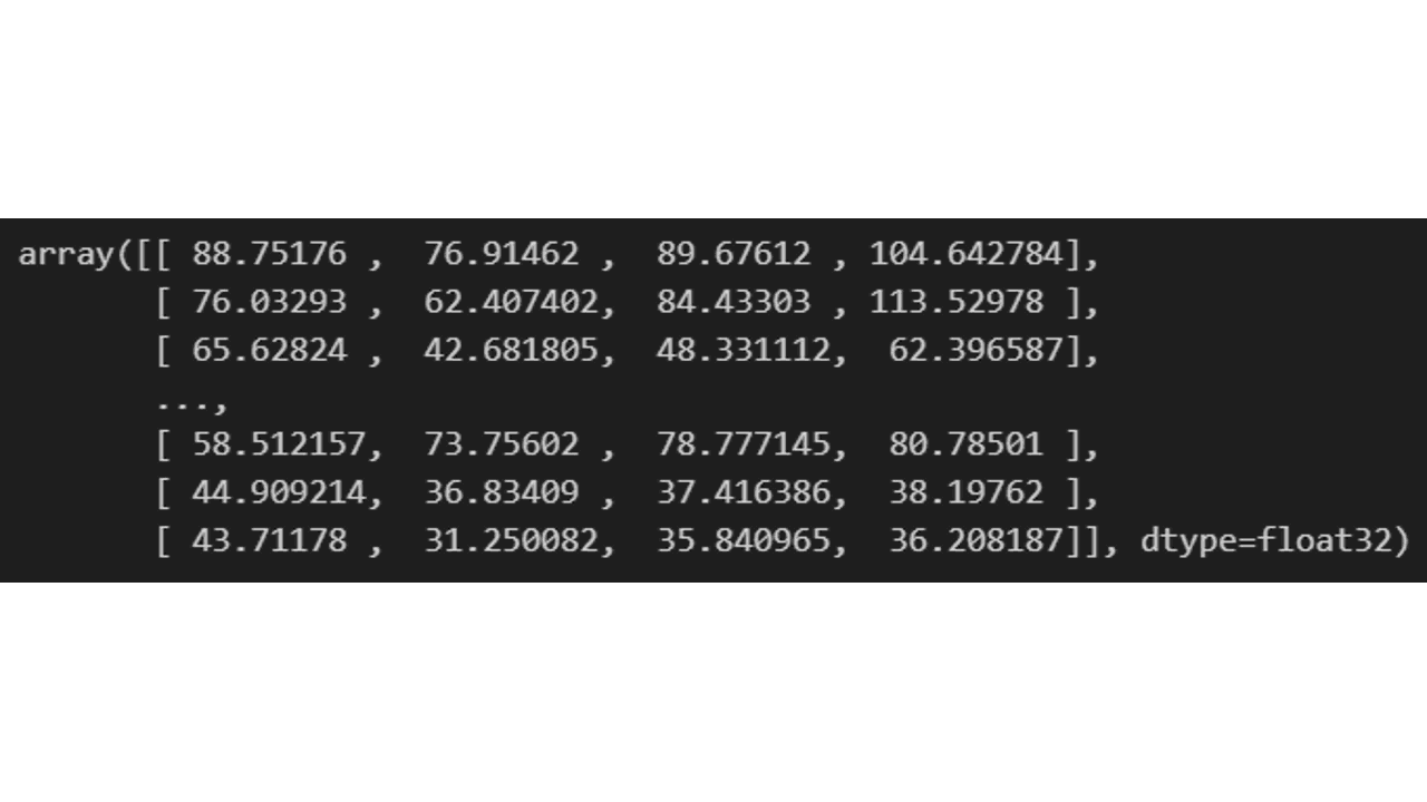
From left to right, the columns represent the predicted values for ‘pm’, ‘stator_yoke’, ‘stator_tooth’, ‘stator_winding’.
Evaluating Model Performance With Scikit-Learn Metrics
Once you’ve made predictions with your model, the next step is to evaluate how well those predictions match the actual values.
For this, we’ll use Scikit-learn’s metrics.
There are many different metrics we could use, as the same ones from single-output regression apply here, but in this tutorial, we’ll focus on Mean Absolute Error (MAE) and Root Mean Squared Error (RMSE).
First, let’s import the necessary functions:
from sklearn.metrics import mean_absolute_error, mean_squared_error
Mean Absolute Error (MAE)
MAE is the average of the absolute differences between the predicted and actual values.
We can calculate MAE in Python using the mean_absolute_error function:
mae = mean_absolute_error(y_test, y_pred)
print(f"Mean Absolute Error: {mae}")
Root Mean Squared Error (RMSE)
RMSE is the square root of the average of the squared differences between the predicted and actual values.
It’s more sensitive to large errors than MAE, meaning it punishes large errors more.
We can calculate RMSE in Python using the mean_squared_error function with squared=False:
rmse = mean_squared_error(y_test, y_pred, squared=False)
print(f"Root Mean Squared Error: {rmse}")
And that’s it!
You’ve now successfully trained, made predictions and evaluated a multi-output regression model with XGBoost in Python.
To improve your model from here, check out my XGBoost hyperparameter tuning tutorial.