
Many people find the initial setup of CatBoost a bit daunting.
Perhaps you’ve heard about its ability to work with categorical features without any preprocessing, but you’re feeling stuck on how to take the first step.
In this step-by-step tutorial, I’m going to simplify things for you.
After all, it’s just another gradient boosting library to have in your toolbox.
We’ll walk you through the process of installing CatBoost, loading your data, and setting up a CatBoost classifier.
Along the journey, we’ll also cover how to divide your data into a training set and a test set, how to manage imbalanced data, and how to train your model on a GPU.
By the end of this guide, you’ll be ready and confident to use CatBoost for your own binary classification projects. So, let’s get started!
Installing CatBoost In Python
There are two main ways to install CatBoost in Python: using pip and conda.
If you prefer using pip, you can install CatBoost by running the following command in your terminal:
pip install catboost
If you prefer using conda, you can install it by running:
conda install -c conda-forge catboost
Make sure you have either pip or conda installed in your Python environment before running these commands.
Once you’ve successfully installed CatBoost, you’re ready to move on to the next step: loading your data.
Loading The Data
We’ll be using the Adult Dataset. You can download it from Kaggle.
This is a well-known dataset that contains demographic information about the US population.
The goal is to predict whether a person makes over $50,000 a year.
CatBoost’s claim to fame is that it can handle categorical features without any preprocessing, so I picked this dataset because it has a mix of categorical and numerical features.
We’ll use the pandas library to load our data.
First, let’s import the necessary libraries:
import pandas as pd
from sklearn.model_selection import train_test_split
Next, let’s load the data.
We’ll use the pandas read_csv function to load the data.
data = pd.read_csv(data_path)
| age | workclass | fnlwgt | education | education.num | marital.status | occupation | relationship | race | sex | capital.gain | capital.loss | hours.per.week | native.country | income |
|---|---|---|---|---|---|---|---|---|---|---|---|---|---|---|
| 90 | ? | 77053 | HS-grad | 9 | Widowed | ? | Not-in-family | White | Female | 0 | 4356 | 40 | United-States | <=50K |
| 82 | Private | 132870 | HS-grad | 9 | Widowed | Exec-managerial | Not-in-family | White | Female | 0 | 4356 | 18 | United-States | <=50K |
| 66 | ? | 186061 | Some-college | 10 | Widowed | ? | Unmarried | Black | Female | 0 | 4356 | 40 | United-States | <=50K |
| 54 | Private | 140359 | 7th-8th | 4 | Divorced | Machine-op-inspct | Unmarried | White | Female | 0 | 3900 | 40 | United-States | <=50K |
| 41 | Private | 264663 | Some-college | 10 | Separated | Prof-specialty | Own-child | White | Female | 0 | 3900 | 40 | United-States | <=50K |
Now we have our data loaded and ready to go.
The next step is to split our data into a training set and a test set.
Let’s use the train_test_split function from the sklearn.model_selection module.
We will split the data into 80% for training and 20% for testing.
X = data.drop('income', axis=1)
y = data['income']

X_train, X_test, y_train, y_test = train_test_split(X, y, test_size=0.2, random_state=42)
In the code above, X is our feature set and y is our target variable which is ‘income’ in this case.
We now have our data split into training and testing sets, and we’re ready to train our CatBoost classifier.
Notice how we don’t have to do any preprocessing for numerical or categorical features.
Training A CatBoost Classifier
The CatBoost library provides a class CatBoostClassifier for binary and multiclass classification tasks.
By default, it uses hyperparameter values that are generally effective for a wide range of datasets.
Still, I recommend you to tune the hyperparameters for your specific dataset to get the best performance.
Let’s import the required library and create an instance of the CatBoostClassifier:
from catboost import CatBoostClassifier

cat_features = X_train.select_dtypes(include=['object']).columns.tolist()
model = CatBoostClassifier(cat_features=cat_features)
The classifier optimizes the Logloss function, also known as cross-entropy loss.
It’s the most common loss function used for binary classification tasks.
Encoding Categorical Features
By default, CatBoost uses one-hot encoding for categorical features with a small number of different values.
For features with high cardinality (like ZIP codes), CatBoost uses a more complex encoding, including likelihood encoding and categorical level counts.
We just need to specify the categorical feature column names in the cat_features parameter when initializing the CatBoostClassifier.
I selected all the non-numerical features as categorical features in the code above.
Handling Imbalanced Data
CatBoost provides the scale_pos_weight parameter.
This parameter adjusts the cost of misclassifying positive examples. A good default value is the ratio of negative to positive samples in the training dataset.
Just divide the number of negative samples by the number of positive samples and pass the result to the scale_pos_weight parameter:
scale_pos_weight = len(y_train[y_train=='<=50K']) / len(y_train[y_train=='>50K'])
model = CatBoostClassifier(cat_features=cat_features, scale_pos_weight=scale_pos_weight)
Be careful though, as this usually breaks the calibration of the model (how close its predicted probabilities are to the true occurrences of the class).
Our data is not terribly imbalanced, so I’ll not use this parameter in this example.
Training On A GPU
Finally, CatBoost allows you to train your model on a GPU.
This can significantly speed up the training process, especially for large datasets.
To enable GPU training, set the task_type parameter to ‘GPU’ when initializing the CatBoostClassifier:
model = CatBoostClassifier(cat_features=cat_features, task_type='GPU')
Finally, let’s train our model on the training data:
model.fit(X_train, y_train)
With this, our CatBoost classifier is trained and ready to make predictions.
Making Predictions With CatBoost
There are two types of predictions we can make: class predictions and probability predictions.
Class Predictions
In this case, the model predicts the class label directly. It does this by setting all examples where the probability of the positive class is greater than 0.5 to 1 and the rest to 0.
class_predictions = model.predict(X_test)
In the above code, model.predict() is used to make class predictions on the test data X_test.
Predicting Probabilities
Sometimes, we might be interested in the probabilities of each class rather than the class itself.
This is useful when we want to have a measure of the confidence of the model in its predictions, use it in a downstream task, or select a custom threshold for the positive class.
CatBoost allows us to predict these probabilities using the predict_proba method:
probability_predictions = model.predict_proba(X_test)
In the above code, model.predict_proba() is used to predict class probabilities.
The output is a 2D array, where the first element of each pair is the probability of the negative class (0) and the second element is the probability of the positive class (1).
Now that we know how to make predictions, let’s move on to evaluate the performance of our model.
Evaluating Model Performance
We’ll use several metrics for this: Log Loss, ROC AUC, and a classification report.
First, let’s import the necessary functions from the sklearn.metrics module:
from sklearn.metrics import log_loss, roc_auc_score, classification_report
Log Loss
Log Loss measures how well a model can guess the true probability of each class.
As it’s the one directly optimized by CatBoost, it tends to be a good measure of the model’s performance.
Lower log loss means better predictions.
It’s not adequate if you are using scale_pos_weight to handle imbalanced data. In that case, you should use ROC AUC instead.
log_loss_value = log_loss(y_test, probability_predictions[:,1])
print(f'Log Loss: {log_loss_value}')
We use probability_predictions[:,1] to get the probability of the positive class (1), as log loss works with probabilities, not class labels.
ROC AUC
ROC AUC (Receiver Operating Characteristic Area Under the Curve) is a performance measurement for classification problems where you are more interested in how well the model predicts the positive examples.
Higher AUC means a better model.
roc_auc = roc_auc_score(y_test, probability_predictions[:,1])
print(f'ROC AUC: {roc_auc}')
Just like before, we need to pass the probability of the positive class (1) to the roc_auc_score function.
Classification Report
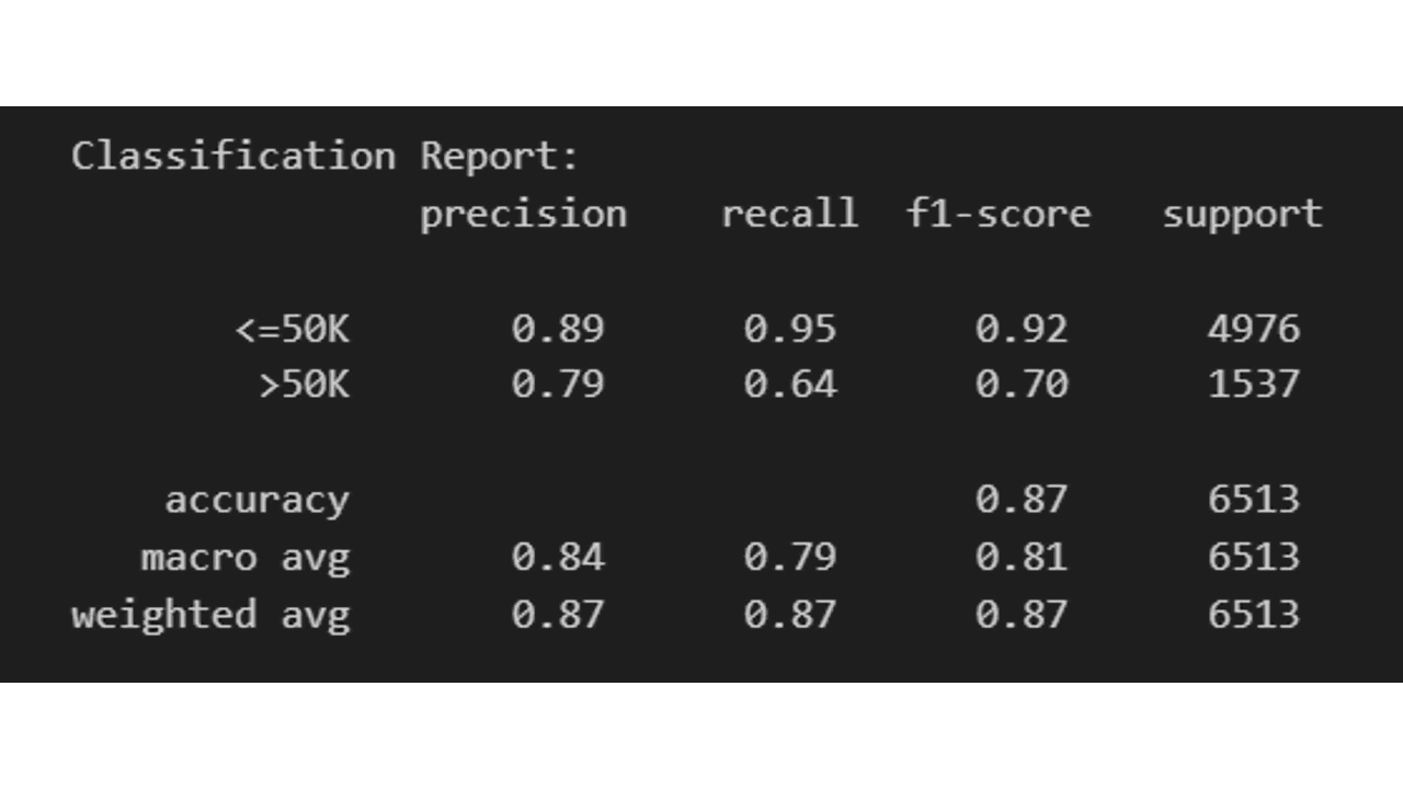
A classification report displays the precision, recall, F1, and support scores for each class and for the whole model.
class_report = classification_report(y_test, class_predictions)
print(f'Classification Report:\n {class_report}')
By evaluating these metrics, you can get a good understanding of how well your CatBoost classifier performs on your binary classification task.