
Multiclass classification is a machine learning task where the output can belong to more than two classes.
In other words, it can sort data into multiple categories.
For example, a piece of fruit can be classified as an ‘apple’, ‘banana’, or ‘cherry’. Or, a car can be classified as ‘sedan’, ‘SUV’, or ’truck’.
Just like binary classification, we can use a variety of algorithms to classify the data points into these multiple categories.
These algorithms include logistic regression, decision trees, random forest, support vector machines, and gradient boosting algorithms like XGBoost.
XGBoost, short for eXtreme Gradient Boosting, is a popular machine learning algorithm in the field of structured or tabular data.
In the next sections, we’ll dive into how to use XGBoost for multiclass classification in Python.
We’ll use the Red Wine dataset. It contains 11 features that describe the chemical properties of different wines and a quality score, that goes from 3 to 8, for each.
Let’s get started!
Installing XGBoost In Python
Before we can start using XGBoost, we need to install it.
XGBoost can be installed using pip, which is a package manager for Python.
To install it, you can use the following command in your terminal:
pip install xgboost
If you are using a Jupyter notebook, you can run this command in a code cell by prefixing it with an exclamation mark:
!pip install xgboost
You can do it using conda and mamba too:
conda install -c conda-forge xgboost
mamba install -c conda-forge xgboost
After running this command, XGBoost should be installed and ready to use.
You can check if it’s installed correctly by importing it in your Python script:
import xgboost as xgb
If this command runs without any errors, congratulations! You have successfully installed XGBoost.
Now, let’s move on to the next section where we will discuss the loss functions for multiclass classification.
Objective (Loss) Functions For Multiclass Classification
In machine learning, the objective function, also known as the loss function, is used to measure the difference between the predicted and actual outcomes.
It guides the model on the path it has to take during training to reach the optimal solution.
Sometimes it’s the same as the evaluation metric, but it doesn’t have to be.
For multiclass classification, XGBoost provides two objective functions:
multi:softmax
When you use multi:softmax, you’re telling the algorithm that there are more than two classes to sort the data into.
When using the scikit-learn API (like we will do here), you don’t need to specify the number of classes as an argument, but you must ensure that your classes start from 0 and go up to the number of classes minus 1.
This will be clearer in the code example below.
This objective function only outputs the class with the highest probability, instead of the probability of each class.
multi:softprob
The multi:softprob is another objective function in XGBoost, also used for multiclass classification problems.
The difference is that instead of just giving the final class as output, multi:softprob gives the probability of the data belonging to each class.
So, for our fruit example, multi:softprob would give the probabilities of it being an apple, banana, or cherry.
This is useful when you want to know not just the final decision, but also how confident the algorithm is in its decision.
When in doubt, use multi:softprob, as it gives you everything that multi:softmax does and more.
Loading The Data
To load the data, we’ll use the pandas library, which is a powerful data handling library in Python.
If you don’t have it installed, you can do so using pip:
pip install pandas
Now, let’s load the Red Wine dataset.
The dataset is available as a CSV file on Kaggle.
We’ll use the pandas function read_csv() to load the data into a DataFrame.
import pandas as pd

# Load the data
data = pd.read_csv('winequality-red.csv')

# Display the first few rows of the data
data.head()
| fixed acidity | volatile acidity | citric acid | residual sugar | chlorides | free sulfur dioxide | total sulfur dioxide | density | pH | sulphates | alcohol | quality |
|---|---|---|---|---|---|---|---|---|---|---|---|
| 7.4 | 0.7 | 0 | 1.9 | 0.076 | 11 | 34 | 0.9978 | 3.51 | 0.56 | 9.4 | 5 |
| 7.8 | 0.88 | 0 | 2.6 | 0.098 | 25 | 67 | 0.9968 | 3.2 | 0.68 | 9.8 | 5 |
| 7.8 | 0.76 | 0.04 | 2.3 | 0.092 | 15 | 54 | 0.997 | 3.26 | 0.65 | 9.8 | 5 |
| 11.2 | 0.28 | 0.56 | 1.9 | 0.075 | 17 | 60 | 0.998 | 3.16 | 0.58 | 9.8 | 6 |
| 7.4 | 0.7 | 0 | 1.9 | 0.076 | 11 | 34 | 0.9978 | 3.51 | 0.56 | 9.4 | 5 |
The head() function is used to get the first n rows. By default, it returns the first 5 rows of the DataFrame.
Now that we have loaded our data, we can move on to training our XGBoost model.
Training XGBoost With The Scikit-Learn API
XGBoost integrates smoothly with the Scikit-Learn library, which provides a consistent API for many different machine learning algorithms in Python.
Before we start training, we need to prepare our data.
We’ll separate our target variable (quality) from the rest of the dataset and split the data into training and test sets.
The original quality column contains values from 3 to 8, so we need to subtract the minimum value from this column to make it start from 0.
from sklearn.model_selection import train_test_split

# Separate target variable
X = data.drop('quality', axis=1)
y = data['quality'] - data['quality'].min()

# Split the data into training and test sets
X_train, X_test, y_train, y_test = train_test_split(X, y, test_size=0.2, random_state=42)
Now, let’s train our XGBoost model.
We’ll use the XGBClassifier class from the XGBoost library.
from xgboost import XGBClassifier

# Create an instance of the XGBClassifier
model = XGBClassifier(objective='multi:softprob')

# Fit the model to the training data
model.fit(X_train, y_train)
If you have used Scikit-Learn before, this should look very familiar.
The fit() function trains the model on the training data.
We pass the features (X_train) and the target (y_train) as parameters to this function.
Now that our model is trained, we can use it to make predictions.
Making Predictions
There are two ways to make predictions using XGBoost that you should be aware of:
Class Predictions
If you want to predict the most likely class of an instance, directly, you can use the predict() function.
# Make class predictions
y_pred = model.predict(X_test)

array([2, 2, 2, 2, 3, 2, 2, 2, 3, 3, 4, 2, 3, 2,... ])
In this case, the model will return the class with the highest probability for each instance.
Predicting Probabilities
Most of the time, we want to know the probabilities that an instance belongs to each class, so we understand how confident the model is in its predictions.
Having the most likely class predicted with 90% confidence is very different from having it predicted with 51%.
The predict_proba() function returns the probabilities for each class.
# Predict probabilities
y_pred_proba = model.predict_proba(X_test)

array([[3.8726095e-05, 1.6520983e-04, 8.5571223e-01, 1.4203377e-01,
        1.9999363e-03, 5.0116490e-05],
       [7.2868759e-05, 7.5193483e-04, 9.8880708e-01, 1.0272802e-02,
        3.8626931e-05, 5.6695393e-05],
        ...])
From left to right, the columns represent the probabilities of the instance belonging to each class.
As expected, each row adds up to 1.
In the next section, we’ll evaluate the performance of our model.
This will give us an idea of how well our model is doing.
Evaluating Model Performance
Evaluating the performance of a model is a crucial step in machine learning.
It helps us understand how well our model is doing and where it can be improved.
Let’s look at some of the ways we can do it.
score function
This is the simplest way to get an evaluation of your model over a dataset.
In XGBoost, it returns the mean accuracy on the given test data and labels.
# Calculate accuracy
accuracy = model.score(X_test, y_test)
print("Accuracy: %.2f%%" % (accuracy * 100.0))
Using Scikit-learn Evaluation Metrics
Scikit-learn provides several functions to calculate metrics such as precision, recall, F1 score, and Log Loss.
To use Log Loss we need to get the probabilities for each class.
from sklearn.metrics import log_loss

# Calculate log loss
log_loss(y_test, y_pred_proba)
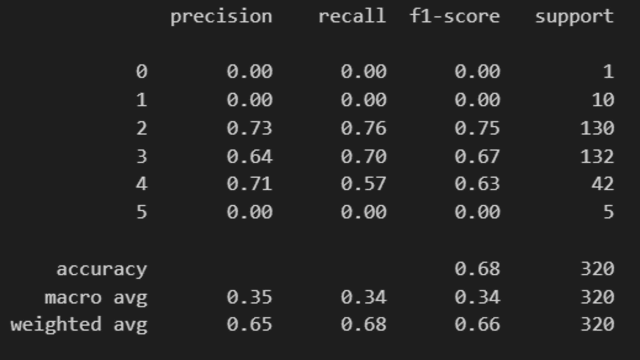
The classification_report() function prints the precision, recall, F1-score and support for each class.
For this function, we need to pass the class predictions, not the probabilities.
from sklearn.metrics import classification_report

# Print classification report
print(classification_report(y_test, y_pred))
Remember, no single metric can tell the whole story.
It’s important to look at multiple metrics and understand what they mean in the context of your specific problem.
Permutation Feature Importance
After training a model, it’s often useful to understand the importance of each feature in making predictions.
This can help us gain insights into the problem and potentially simplify the model by removing irrelevant features.
XGBoost provides a built-in methods to calculate feature importance, which are based on factors like the number of times a feature is used to split the data and the average gain of the splits.
However, this method has some limitations, especially for data with correlated features.
An alternative approach is to use permutation feature importance, which is a model-agnostic technique that can be applied to any machine learning model.
The basic idea behind permutation feature importance is to measure the increase in the model’s prediction error after permuting (shuffling) the values of a feature on an unseen dataset.
If a feature is important, shuffling its values should significantly increase the model’s error.
Conversely, if a feature is not important, shuffling its values should have little to no effect on the model’s error.
Here’s how we can calculate permutation feature importance for our XGBoost model:
from sklearn.inspection import permutation_importance

# Calculate permutation feature importance
result = permutation_importance(
    model, X_test, y_test, scoring='neg_log_loss', n_repeats=10, random_state=42
)

# Get the feature importances and sort them in descending order
feature_importances = pd.Series(result.importances_mean, index=X.columns).sort_values(ascending=False)

# Print the feature importances
print(feature_importances)
| Feature | Importance |
|---|---|
| alcohol | 0.377121 |
| sulphates | 0.280283 |
| volatile acidity | 0.188259 |
| total sulfur dioxide | 0.152310 |
| residual sugar | 0.051633 |
| citric acid | 0.049829 |
| pH | 0.049466 |
| fixed acidity | 0.043403 |
| density | 0.041544 |
| chlorides | 0.021090 |
| free sulfur dioxide | -0.012878 |
The permutation_importance function from scikit-learn takes the following parameters:
model: The trained model for which we want to calculate feature importance.X_test: The feature matrix for the unseen (validation) set.y_test: The target variable for the unseen (validation) set.scoring: The metric to use for measuring the increase in prediction error. We’re using'neg_log_loss'for multiclass classification.n_repeats: The number of times to permute each feature. More repetitions lead to more stable results but take longer to compute.random_state: The seed for the random number generator, to ensure reproducibility.
The function returns a PermutationImportance object, which contains the mean and standard deviation of the increase in prediction error for each feature.
We extract the mean importances using result.importances_mean, create a pandas Series with the feature names as the index, sort the Series in descending order, and print it.
This will give us an ordered list of features, with the most important features at the top and the least important features at the bottom.
Interpreting feature importance can be tricky, and it’s always a good idea to combine it with domain knowledge and other exploratory data analysis techniques.
However, it can be a useful tool for understanding the behavior of your model and potentially improving its performance by removing or downweighting irrelevant features.
And that’s it!
Happy coding!
PS: Check the tutorial on learning to rank with XGBoost next!