
If you are using XGBoost with decision trees as your base model, you don’t need to worry about scaling or normalizing your features.
Decision trees are not sensitive to the scale of the features.
In practice, I have seen very minor differences in score by scaling[features for decision trees, but these are due to numerical computing implementations and not significant in practice.
If you are using XGBoost with linear models as base models, it is a good idea to scale or normalize the features.
This is because linear models are sensitive to the scale of the features when trained with gradient-based methods, and using scaled or normalized features can lead to better performance.
If the scale of the features is very different, the coefficients of the linear model will be influenced more by the features with the larger scales, and the model may have difficulty learning the relationships between the other features and the target variable.
Comparing Decision Tree XGBoost Results With and Without Scaling
Here is a comparison between XGBoost using Decision Trees as the base model with standardized features vs no preprocessing in the famous red wine dataset, which has only numerical features.
import pandas as pd
import numpy as np
from xgboost import XGBRegressor
from sklearn.preprocessing import StandardScaler
from sklearn.model_selection import train_test_split
from sklearn.metrics import mean_squared_error

# Load the red wine dataset
data = pd.read_csv("winequality-red.csv")

# Split the data into features and target
X = data.drop(columns=["quality"])
y = data["quality"]

# Split the data into training and validation sets
X_train, X_val, y_train, y_val = train_test_split(X, y, test_size=0.3, random_state=42)

# Fit an XGBoost model to the training data
xgb_model = XGBRegressor(random_state=42)
xgb_model.fit(X_train, y_train)

# Make predictions on the validation set
xgb_predictions = xgb_model.predict(X_val)

# Calculate the root mean squared error of the model on the validation set
xgb_rmse = np.sqrt(mean_squared_error(y_val, xgb_predictions))

# Print the root mean squared error of the model on the validation set
print("RMSE of XGBoost model without scaling:", xgb_rmse)

# Scale the data using StandardScaler
scaler = StandardScaler()
X_train_scaled = scaler.fit_transform(X_train)
X_val_scaled = scaler.transform(X_val)

# Fit an XGBoost model to the scaled training data
xgb_model_scaled = XGBRegressor(random_state=42)
xgb_model_scaled.fit(X_train_scaled, y_train)

# Make predictions on the scaled validation set
xgb_predictions_scaled = xgb_model_scaled.predict(X_val_scaled)

# Calculate the root mean squared error of the model on the scaled validation set
xgb_rmse_scaled = np.sqrt(mean_squared_error(y_val, xgb_predictions_scaled))

# Print the root mean squared error of the model on the scaled validation set
print("RMSE of XGBoost model with scaling:", xgb_rmse_scaled)
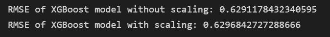
As I said, sometimes there is a difference because of the imperfect nature of numerical computing algorithms, but it’s very small and unlikely to be significant for practical use.
Comparing Linear XGBoost Results With and Without Scaling
It’s a different story when you use XGBoost with base linear models.
Here is the comparison:
import pandas as pd
import numpy as np
from xgboost import XGBRegressor
from sklearn.preprocessing import StandardScaler
from sklearn.model_selection import train_test_split
from sklearn.metrics import mean_squared_error

# Load the red wine dataset
data = pd.read_csv("winequality-red.csv")

# Split the data into features and target
X = data.drop(columns=["quality"])
y = data["quality"]

# Split the data into training and validation sets
X_train, X_val, y_train, y_val = train_test_split(X, y, test_size=0.3, random_state=42)

# Fit an XGBoost model with a linear booster to the training data
xgb_model = XGBRegressor(booster='gblinear', random_state=42)
xgb_model.fit(X_train, y_train)

# Make predictions on the validation set
xgb_predictions = xgb_model.predict(X_val)

# Calculate the root mean squared error of the model on the validation set
xgb_rmse = np.sqrt(mean_squared_error(y_val, xgb_predictions))

# Print the root mean squared error of the model on the validation set
print("RMSE of XGBoost model with a linear booster:", xgb_rmse)

# Scale the data using StandardScaler
scaler = StandardScaler()
X_train_scaled = scaler.fit_transform(X_train)
X_val_scaled = scaler.transform(X_val)

# Fit an XGBoost model with a linear booster to the scaled training data
xgb_model_scaled = XGBRegressor(booster='gblinear', random_state=42)
xgb_model_scaled.fit(X_train_scaled, y_train)

# Make predictions on the scaled validation set
xgb_predictions_scaled = xgb_model_scaled.predict(X_val_scaled)

# Calculate the root mean squared error of the model on the scaled validation set
xgb_rmse_scaled = np.sqrt(mean_squared_error(y_val, xgb_predictions_scaled))

# Print the root mean squared error of the model on the scaled validation set
print("RMSE of XGBoost model with a linear booster and scaling:", xgb_rmse_scaled)

As the results show, XGBoost with a linear booster is much more sensitive to scaling.
When I was running the experiments, the scaled version had the stable score you are seeing in the image, but the unscaled version score kept changing even with random seeds set.
My hypothesis is that due to the numerical instability, the model has trouble converging to a solution, appearing random.
How To Scale Features For Linear XGBoost?
You can use the same methods that are used with linear models outside of XGBoost.
Here are some examples of how to do it:
Standardization
This is, by far, the most common method. It’s the one I used in the comparison.
It involves subtracting the mean of each feature from each value and dividing it by the standard deviation.
This scales the features to have zero mean and unit variance.
Just be careful with outliers as this method can be sensitive to extreme values in the data.
from sklearn.preprocessing import StandardScaler

# Initialize the StandardScaler
scaler = StandardScaler()

# Fit the StandardScaler to the training data
scaler.fit(X_train)

# Use the scaler to transform the training and test sets
X_train_scaled = scaler.transform(X_train)
X_test_scaled = scaler.transform(X_test)
Min-Max Scaling
This method scales the features to a specific range, such as [0, 1] or [-1, 1].
It involves subtracting the minimum value of each feature from each value and dividing it by the range (i.e., the difference between the maximum and minimum values).
from sklearn.preprocessing import MinMaxScaler

# Initialize the MinMaxScaler
scaler = MinMaxScaler()

# Fit the MinMaxScaler to the training data
scaler.fit(X_train)

# Use the scaler to transform the training and test sets
X_train_scaled = scaler.transform(X_train)
X_test_scaled = scaler.transform(X_test)
Normalization
This method scales the features to have a unit norm (i.e., a length of 1 in a multi-dimensional space).
It usually involves dividing each value by the Euclidean norm (also known as the L2 norm) of the feature.
from sklearn.preprocessing import Normalizer

# Initialize the Normalizer
scaler = Normalizer()

# Fit the Normalizer to the training data
scaler.fit(X_train)

# Use the scaler to transform the training and test sets
X_train_scaled = scaler.transform(X_train)
X_test_scaled = scaler.transform(X_test)
Scaling By The Maximum Absolute Value
This is another method for scaling the features that is useful for sparse data.
Sparse data is data that has a many more zeros than other values.
Standardizing sparse data, for example, breaks the sparsity as it replaces the zeros by non-zero values.
This is why it’s recommended to use other methods.
It scales the data to the range [-1, 1] by dividing it by the maximum absolute value of the feature.
from sklearn.preprocessing import MaxAbsScaler

# Initialize the MaxAbsScaler
scaler = MaxAbsScaler()

# Fit the MaxAbsScaler to the training data
scaler.fit(X_train)

# Use the scaler to transform the training and test sets
X_train_scaled = scaler.transform(X_train)
X_test_scaled = scaler.transform(X_test)
How To Select The Best Scaling Method For Linear XGBoost?
As with any other model, the best scaling method will depend on the specific characteristics of your dataset.
Try different scaling methods and see which gets you the best evaluation metric in your validation data.